The Southern Tier of New York, comprising fourteen counties designated as part of Northern Appalachia by the Appalachian Regional Commission (ARC), has long faced significant socioeconomic challenges. These counties have experienced some of the steepest population declines in New York State outside of New York City, driven by prolonged economic restructuring and out-migration (McMahon, 2024; Johnson & Lichter, 2019). Historically reliant on manufacturing, agriculture, and extractive industries, the region has struggled to adapt to post-industrial economic realities. As a result, many communities across the Southern Tier endure persistently high poverty rates and low median incomes relative to national benchmarks (ARC, 2023).
Map of three subregions in Appalachian NY (NY Department of State)
To monitor and address such disparities, the ARC employs its Distressed Areas Classification System, which is traditionally applied at the county level (ARC, 2024). This system designates areas as “distressed” if they exhibit a median family income no greater than 67% of the U.S. average and a poverty rate at least 150% of the national average. While sufficient for broad regional assessments, scholars have noted that county-level classifications risk obscuring critical intra-county variations, particularly in regions marked by sharp spatial heterogeneity (Partridge et al., 2008; Thiede et al., 2017). Applying this framework at the census block group level allows for a more granular understanding of localized socioeconomic distress, capturing neighborhood-level vulnerabilities often masked in aggregate statistics.
This study adopts such a fine-scaled approach by applying the ARC’s criteria at the block group level across the Southern Tier. Beyond mere classification, however, this analysis seeks to model the risk of socioeconomic distress by incorporating key demographic, economic, and spatial predictors. Using a Generalized Linear Mixed Model (GLMM) framework implemented via the glmmTMB package in R, this study not only identifies predictors of distress but also evaluates the spatial adequacy of the ARC’s classification system.
The glmmTMB framework is particularly well-suited for this analysis due to its flexibility in handling binary outcomes, accounting for hierarchical spatial structures, and integrating spatially lagged covariates all of which encompass a methodological advancement increasingly adopted in socioeconomic and public health research (Bivand & Piras, 2015; Brooks et al., 2017; Dormann et al., 2007). Recent studies have leveraged glmmTMB to model spatial patterns of poverty (Jokela et al., 2019) and health disparities (Barrett et al., 2023), highlighting its capacity to address complex data structures characterized by spatial autocorrelation and unobserved heterogeneity.
By combining the ARC’s established distress criteria with predictive modeling, this study aims to (1) assess the underlying risk factors contributing to distress in the Southern Tier, and (2) critically evaluate where the ARC’s classification aligns (or falls short) in capturing the true geography of socioeconomic vulnerability. This approach provides a nuanced understanding of distress that can inform more targeted policy interventions within New York’s Appalachian region.
Materials and Methods
Data
The analysis looked at various socioeconomic variables along with land cover classifications. Specifically, data concerning average family income, poverty rate, people over the age of 16 who hadn’t worked in the previous 12 month period (hereon referred to as “unemployment rate”), average rent, people over the age of 15 who are divorced (hereon referred to as “divorced rate”), and population density were pulled and/or aggregated at the block group, county, and country levels.
Census data was pulled for years between 2009 and 2023. All block group-level data was gathered using the ipumsr package, and all of it originally came from American Community Survey (ACS) 5-year estimates housed by the NHGIS in its IPUMS collection. For distressed status classification, some country-level data for 2009 and 2010 was pulled using the tidycensus package, while the rest of it had to be sourced from governmental reports and news releases since ACS data may not have been readily available for this year at the country-level. Block group-level data was aggregated at the county-level to view changes in these socioeconomic indicators and land cover.
To ensure the uniform block group boundaries across the 14-county study area, the interpolate_pw function within tidycensus was used for population-weighted areal interpolation via centroid assignment (Walker, 2023). The use of scaling factors applied to each individual extensive variable was required to ensure the preservation of total counts across each of the variables by correcting for biases introduced by differing spatial distributions (Gregory, 2002; Goodchild & Lam, 1980; Flowerdew & Green, 1992).
As mentioned previously, the methodology used to determine distressed status of each census tract derives from the Appalachian Regional Commission’s Distressed Areas Classification System. According to the ARC, the key attributes of a distressed census tract are:
A median family income no greater than 67% of the U.S. average.
A poverty rate of 150% of the U.S. average or greater.
Since median family incomes cannot be appropriately interpolated, average family income at the national level was used to determine distressed status of each block group rather than the median.
Land cover data was processed using the terra package. All land cover classifications were grouped into 9 groups (including Developed, Agriculture, Forest, etc.). Zonal statistics were calculated for each class within each block group, and the coverage percentage of each class was calculated for each block group. Developed land ultimately became the only land cover classification that was considered in the predictive model.
Model Using glmmTMB
A logistic generalized linear mixed model was estimated using the glmmTMB package to assess distress risk across the 1,004 uniform block groups. Population density, unemployment rate, average rent, and divorced rate were included as socioeconomic/demographic predictors. Additionally, spatial dependence was accounted for by incorporating a spatially lagged covariate for unemployment rate as a fixed effect in the GLMM model. This approach allows for partial control of spatial autocorrelation within glmmTMB, and was especially necessary given the socioeconomic nature of this study, the expected clustering of socioeconomic conditions, and the expansive study area.
Including time period fixed effects in a glmmTMB model is a common approach to control for unobserved temporal factors that could bias estimates, such as policy changes, economic cycles, or external shocks affecting all units over time (Zuur et al., 2009). This method isolates the impact of key predictors by accounting for systematic variations across different periods within generalized linear mixed models.
Including GEOID as a random effect in a glmmTMB model accounts for unobserved, unit-specific heterogeneity across spatial units, such as census block groups or tracts, allowing the model to control for clustering and repeated measures within geographic areas (Gelman & Hill, 2007). This approach improves inference by addressing potential correlation within groups and capturing latent spatial characteristics not explained by fixed effects. The model assigns each unique block group a random intercept, and these random intercepts represent the baseline log-odds of distress for each block group after accounting for all fixed effects. In other words, this is the unexplained spatial variation - the residual risk attributable to block group-level factors not captured by the model’s included predictors.
Scaling predictor variables in a glmmTMB model is a standard practice to improve model convergence, interpretability, and comparability of effect sizes, especially when predictors are on different scales or have large variances (Schielzeth, 2010). Standardization centers variables around zero and ensures that coefficients represent the effect of a one standard deviation change, facilitating more meaningful interpretation in generalized linear mixed models.
After successfully estimating the GLMM, the DHARMa package was used for diagnostic tests to evaluate the assumptions. The spdep package was used to conduct a Moran’s I test to determine the presence of spatial autocorrelation.
Other Methods
The tidyverse collection of packages was primarily used to easily process a large amount of data. The tigris package was used directly to pull study counties to create a map of the study area, as well as to pull block-level data for use as the weights in the interpolation process. The sf package helped with processing spatial features, including data pulled from the ACS. The maps and general plots were created using ggplot2. The gt package allowed for the creation of better looking tables.
Data Gathering and Processing
Map of Study Area
The map below shows the 14 counties in New York’s Southern Tier (Allegany, Broome, Cattaraugus, Chautauqua, Chemung, Chenango, Cortland, Delaware, Otsego, Schoharie, Schuyler, Steuben, Tioga, and Tompkins) and all 1,004 block groups (in 2020-2023).
Code
# set directories in cwd in which to store datadata_download_path <-'data/'nhgis_data_dir <-paste(data_download_path, 'nhgis/', sep ='')mrlc_data_dir <-paste(data_download_path, 'mrlc/', sep ='')boundaries_data_dir <-paste(data_download_path, 'boundaries/', sep ='')# set vector of southern tier countiessouthern_tier_counties =c('Allegany', 'Broome', 'Cattaraugus', 'Chautauqua', 'Chemung', 'Chenango', 'Cortland', 'Delaware', 'Otsego', 'Schoharie', 'Schuyler', 'Steuben', 'Tioga', 'Tompkins')# get study geographies, city and town boundaries, and basemap focused on ny stateny_state <-states(cb =TRUE, year =2020) %>%filter(NAME =='New York')# list of county FIPScounty_fips <-c("003", "007", "009", "013", "015", "017", "023", "025", "077", "095", "097", "101", "107", "109")# get southern tier county boundariesstudy_counties <-counties(state ='NY', cb =TRUE, year =2020) %>%filter(NAME %in% southern_tier_counties)# get block groups in southern tierstudy_bgs <-block_groups(state ='NY', year =2020) %>%filter(COUNTYFP %in% county_fips)# get basemap of NYbase_ny <-basemap_raster(ext = ny_state, map_service ='carto', map_type ='light', verbose =FALSE)# get villages and citiesst_civil <-st_read('data/boundaries/NYS_Civil_Boundaries.geojson', quiet =TRUE) %>%filter(COUNTY %in% southern_tier_counties) %>%st_transform(crs =26918)st_cities <-st_read('data/boundaries/NYS_City_Boundaries.geojson', quiet =TRUE) %>%filter(COUNTY %in% southern_tier_counties) %>%st_transform(crs =26918)# filter out certain villages, transform, and get centroidscivil <- st_civil %>%st_transform(crs =26918) %>%st_centroid() %>%select(NAME, geometry) %>%filter(NAME %in%c("Alfred", "Wellsville", "Bath", "Cooperstown", "Watkins Glen", "Sidney", "Delhi", "Waverly", "Owego", "Cobleskill", "Hancock"))# transform cities and get centroidscities <- st_cities %>%st_transform(crs =26918) %>%st_centroid() %>%select(NAME, geometry)# plot block groups, counties, and names of cities and villagesst_map <-ggplot() +geom_sf(data = study_bgs %>%st_transform(crs ='EPSG:26918'), color ='lightpink', fill ='white', size =2.5) +geom_sf(data = study_counties %>%st_transform(crs ='EPSG:26918'), color ='black', fill =NA, size =2) +geom_sf_text(data = cities, aes(label = NAME), angle =22.5, size =4) +geom_sf_text(data = civil, aes(label = NAME), angle =-22.5, size =3.25) +labs(title ='NY Southern Tier Counties and Block Groups',subtitle ='Block Groups as of 2020') +theme_map() +theme(plot.margin =margin(10, 10, 10, 10),legend.position ='none' ) +coord_sf(expand =FALSE)st_map
Download and Process All Required Data
Data at the U.S. level is pulled first. This data is used in determining distress status of each block group. Next, block group-level data is pulled and pre-processed.
ACS Data
U.S. Data
Create collection of distressed indicator-related data at U.S. level for each year between 2009 and 2023.
Code
# set US data for 2009 and 2010us_data.2009<-data.frame(Name ='United States',year =2009,tot_pop =301461533,pct_below_poverty =0.143,median_income =64000,per_capita_income =39307,pct_over_16_didnt_work =0.2133001) %>%as_tibble()us_data.2010<-data.frame(Name ='United States',year =2010,tot_pop =312471327,pct_below_poverty =0.153,median_income =64400,per_capita_income =40557,pct_over_16_didnt_work =0.223817) %>%as_tibble()# pull US data from ACS for 2011-2023us_data.2011_2023 <-map2(2011:2023, rep('us', times =13), get_acs_data) %>%bind_rows() %>%rename_with(~str_replace(., 'E$', ''), .cols =ends_with('E')) %>%select(-ends_with('M')) %>%mutate(Name ='United States',pct_below_poverty = tot_below_poverty / tot_pop,pop_over_16_didnt_work = males_didnt_work + females_didnt_work,pct_over_16_didnt_work = pop_over_16_didnt_work / tot_pop_over_16,pop_over_15_divorced = males_divorced + females_divorced,pct_divorced = pop_over_15_divorced / tot_pop_over_15 ) %>%select(Name, year, tot_pop, per_capita_income, pct_over_16_didnt_work, median_income, pct_below_poverty, pct_divorced) %>%as_tibble()# combine data into single tibbleus_data <-bind_rows(us_data.2009, us_data.2010, us_data.2011_2023)
Block Group Data
Define an extract to submit to NHGIS, then download, load, and process data.
Download Set-Up
Code
# set datasets to pull block and block group data from (2009-2023)datasets <-c('2005_2009_ACS5a', '2006_2010_ACS5a', '2007_2011_ACS5a', '2008_2012_ACS5a', '2009_2013_ACS5a', '2010_2014_ACS5a','2011_2015_ACS5a', '2012_2016_ACS5a', '2013_2017_ACS5a','2014_2018_ACS5a', '2015_2019_ACS5a', '2016_2020_ACS5a','2017_2021_ACS5a', '2018_2022_ACS5a', '2019_2023_ACS5a')# extract specifications with variables and geographic level (block group) for each datasetbg_dataset_spec <-map( datasets,~ds_spec( .x,#data_tables = c('B01003', 'B11001', 'B17021', 'B19127'),data_tables =c('B01003', 'B17021', 'B19101', 'B19127', 'B19301', 'B23022', 'B25001', 'B25004', 'B25008', 'B25065', 'B11001', 'B25010', 'B12001'),geog_levels ='blck_grp' ))# set list of shapefiles to include in extractbg_shps <-c('360_blck_grp_2000_tl2009', '360_blck_grp_2010_tl2010','360_blck_grp_2011_tl2011', '360_blck_grp_2012_tl2012','360_blck_grp_2013_tl2013', '360_blck_grp_2014_tl2014','360_blck_grp_2015_tl2015', '360_blck_grp_2016_tl2016','360_blck_grp_2017_tl2017', '360_blck_grp_2018_tl2018','360_blck_grp_2019_tl2019', '360_blck_grp_2020_tl2020','360_blck_grp_2021_tl2021', '360_blck_grp_2022_tl2022','360_blck_grp_2023_tl2023')########################################################## RUN THIS CODE THE FIRST TIME, COMMENT IT OUT AFTERWARDS########################################################## # define extract used to pull from NHGIS# bg_extract <- define_extract_nhgis(# description = 'Block Groups ACS Data and NY Shapefiles (2009-2023)',# datasets = bg_dataset_spec,# geographic_extents = '360',# shapefiles = bg_shps# )# # # create data pull and store it in your account# final_bg_extract <- wait_for_extract(submit_extract(bg_extract))# # # download files to computer# bg_nhgis_files <- download_extract(final_bg_extract, download_dir = nhgis_data_dir)#########################################################
Load and Process Block Group Data
Code
# get zip files# CHANGE THIS ACCORDINGLY TO REFLECT YOUR FILE STRUCTUREnhgis_bg_data <-list.files(path = nhgis_data_dir, pattern ='csv', full.names =TRUE)[[4]]nhgis_bg_shps <-list.files(path = nhgis_data_dir, pattern ='shape', full.names =TRUE)[[4]]########################################## load tabular data for all block groups########################################## initiatlize list of block group data for each yearbg_data_yrs <-c()# iterate over each year# filter for relevant study variables, process the data, then merge data# with respective spatial filefor (yr in2009:2023) {#print(as.character(yr))# load and pre-process data d <-read_nhgis(nhgis_bg_data, file_select =matches(as.character(yr))) %>% .[cumall(!('NAME_M'==colnames(.)))] %>%mutate(YEAR =str_split(YEAR, '-', simplify =TRUE)[,2],COUNTY =str_split(COUNTY, ' ', simplify =TRUE)[,1]) %>%filter(COUNTY %in% southern_tier_counties)# load shapefile s <-read_ipums_sf(nhgis_bg_shps, file_select =matches(as.character(yr)))# 2009if (yr ==2009) { d <- d %>%mutate(GEOID =str_split(GEOID, 'US', simplify =TRUE)[,2]) %>%mutate_at(vars(GEOID), as.numeric) %>%rename(year = YEAR, county = COUNTY, name = NAME_E,tot_pop =39, tot_hhs =40, tot_families =41,tot_pop_over_15 =49, males_divorced =58, females_divorced =67,tot_pop_pov_count =68, pop_in_poverty =69, agg_fam_income =120,per_capita_income =121, pop_over_16 =122, males_didnt_work =146,females_didnt_work =170, tot_housing_units =171, vacant_housing_units =172,renter_occ_housing_units =182, agg_gross_rent =186 ) %>% .[,c(2, 8, 37:41, 49, 58, 67:69, 120:122, 146, 170:172, 182, 186)] %>%relocate(GEOID, .before = year) %>%relocate(c(county, year), .after = name) s <- s %>%mutate(GEOID =as.numeric(paste(STATEFP00, COUNTYFP00, TRACTCE00, BLKGRPCE00, sep=''))) %>%filter(GEOID %in% (d$GEOID)) %>%select(GEOID, geometry) %>%st_transform(crs =st_crs(study_bgs)) } elseif (yr ==2010) { # 2010 d <- d %>%mutate(GEOID =str_split(GEOID, 'US', simplify =TRUE)[,2]) %>%mutate_at(vars(GEOID), as.numeric) %>%rename(year = YEAR, county = COUNTY, name = NAME_E,tot_pop =41, tot_hhs =42, tot_families =43,tot_pop_over_15 =51, males_divorced =60, females_divorced =69,tot_pop_pov_count =70, pop_in_poverty =71, agg_fam_income =122,per_capita_income =123, pop_over_16 =124, males_didnt_work =148,females_didnt_work =172, tot_housing_units =173, vacant_housing_units =174,renter_occ_housing_units =184, agg_gross_rent =188 ) %>% .[,c(2, 8, 37, 40:43, 51, 60, 69:71, 122:124, 148, 172:174, 184, 188)] %>%relocate(GEOID, .before = year) %>%relocate(c(county, year), .after = name) s <- s %>%rename(GEOID =`GEOID10`) %>%mutate(across(GEOID, as.numeric)) %>%filter(GEOID %in% (d$GEOID)) %>%select(GEOID, geometry) %>%st_transform(crs =st_crs(study_bgs)) } elseif (yr >=2011& yr <=2020) { # 2011 to 2020 d <- d %>%mutate(GEOID =str_split(GEOID, 'US', simplify =TRUE)[,2]) %>%mutate(across(GEOID, as.numeric)) %>%rename(year = YEAR, county = COUNTY, name = NAME_E,tot_pop =42, tot_hhs =43, tot_families =44,tot_pop_over_15 =52, males_divorced =61, females_divorced =70,tot_pop_pov_count =71, pop_in_poverty =72, agg_fam_income =123,per_capita_income =124, pop_over_16 =125, males_didnt_work =149,females_didnt_work =173, tot_housing_units =174, vacant_housing_units =175,renter_occ_housing_units =185, agg_gross_rent =189 ) %>% .[,c(2, 8, 38, 41:44, 52, 61, 70:72, 123:125, 149, 173:175, 185, 189)] %>%relocate(GEOID, .before = year) %>%relocate(c(county, year), .after = name) s <- s %>%filter(GEOID %in% (d$GEOID)) %>%mutate(across(GEOID, as.numeric)) %>%select(GEOID, geometry) %>%st_transform(crs =st_crs(study_bgs)) } elseif (yr >=2021& yr <=2022) { # 2021 to 2022 d <- d %>%mutate(GEO_ID =str_split(GEO_ID, 'US', simplify =TRUE)[,2]) %>%mutate_at(vars(GEO_ID), as.numeric) %>%rename(year = YEAR, county = COUNTY, name = NAME_E,tot_pop =43, tot_hhs =44, tot_families =45,tot_pop_over_15 =53, males_divorced =62, females_divorced =71,tot_pop_pov_count =72, pop_in_poverty =73, agg_fam_income =124,per_capita_income =125, pop_over_16 =126, males_didnt_work =150,females_didnt_work =174, tot_housing_units =175, vacant_housing_units =176,renter_occ_housing_units =186, agg_gross_rent =190 ) %>% .[,c(2, 8, 38, 42:45, 53, 62, 71:73, 124:126, 150, 174:176, 186, 190)] %>%rename(GEOID = GEO_ID) %>%relocate(GEOID, .before = year) %>%relocate(c(county, year), .after = name) s <- s %>%filter(GEOID %in% (d$GEOID)) %>%mutate(across(GEOID, as.numeric)) %>%select(GEOID, geometry) %>%st_transform(crs =st_crs(study_bgs)) } else { # 2023 d <- d %>%mutate(GEO_ID =str_split(GEO_ID, 'US', simplify =TRUE)[,2]) %>%mutate_at(vars(GEO_ID), as.numeric) %>%rename(year = YEAR, county = COUNTY, name = NAME_E,tot_pop =42, tot_hhs =43, tot_families =44,tot_pop_over_15 =52, males_divorced =61, females_divorced =70,tot_pop_pov_count =71, pop_in_poverty =72, agg_fam_income =123,per_capita_income =124, pop_over_16 =125, males_didnt_work =149,females_didnt_work =173, tot_housing_units =174, vacant_housing_units =175,renter_occ_housing_units =185, agg_gross_rent =189 ) %>% .[,c(2, 8, 37, 41:44, 52, 61, 70:72, 123:125, 149, 173:175, 185, 189)] %>%rename(GEOID = GEO_ID) %>%relocate(GEOID, .before = year) %>%relocate(c(county, year), .after = name) s <- s %>%filter(GEOID %in% (d$GEOID)) %>%mutate(across(GEOID, as.numeric)) %>%select(GEOID, geometry) %>%st_transform(crs =st_crs(study_bgs)) }# convert year and data columns to numeric, then change negative and NA values to 0 data <- d %>%mutate(across(c(tot_pop:agg_gross_rent), as.numeric),across(c(tot_pop:agg_gross_rent), ~ifelse(is.na(.) | . <0| . =='.', '0', .))) data[is.na(data)] <-0# join spatial features with data then transform to NAD83 full_data <-inner_join(s, data, by ='GEOID') %>%relocate(geometry, .after =last_col()) %>%st_transform(crs =st_crs(study_bgs))# add to bg_data_yrs and move onto the next year after doing this bg_data_yrs[[as.character(yr)]] <- full_data}# combine block group data into single dataframest_bgs <-bind_rows(bg_data_yrs) %>%mutate(across(c(GEOID, year, agg_fam_income, per_capita_income, agg_gross_rent), as.numeric),pop_over_16_didnt_work = males_didnt_work + females_didnt_work ) %>%relocate(geometry, .after =last_col())st_bgs[is.na(st_bgs)] <-0
Population-Weighted Areal Interpolation and Distressed Status Determination
Apply population-weighted areal interpolation using centroid assignment to the 2009 - 2019 block group boundaries and ensure that they follow the 2020 boundaries. Estimate all data by applying a scaling factor to each variable after interpolation. Merge all the data together, recombine with 2020-2023 data, then calculate remaining variables.
Code
# isolate post-2020 block group datast_bgs.post_2020 <- st_bgs %>%filter(year >=2020) %>%select(-name) %>%st_make_valid()# get only 2020 block groupsst_bgs.2020<- st_bgs %>%filter(year ==2020) %>%st_make_valid()# get 2020 blocks to use as weights in interpolationst_blocks.2020<- tigris::blocks(state ='NY', year =2020) %>%filter(COUNTYFP20 %in% county_fips) %>%st_make_valid()# get list of variables to scalevars_to_scale <-c("tot_pop", "tot_hhs", "tot_families", "tot_pop_over_15", "males_divorced", "females_divorced", "tot_pop_pov_count", "pop_in_poverty", "agg_fam_income", "agg_income", "pop_over_16", "males_didnt_work", "females_didnt_work", "tot_housing_units", "vacant_housing_units", "renter_occ_housing_units", "agg_gross_rent", "pop_over_16_didnt_work")# interpolate block groups boundaries and new boundary data for each year,# then store in interpolated data listinterpolated_data <-lapply(2009:2019, interpolate_data)# bind interpolated data togetherst_interpolated.pre_2020 <-bind_rows(interpolated_data) %>%relocate(geometry, .after =last_col())# bind yearly interpolated data into single dataframe# calculate total divorced population and determine distressed statusst_bgs_final <-bind_rows(st_interpolated.pre_2020, st_bgs.post_2020 %>%mutate(year =as.numeric(year))) %>%left_join(us_data %>%select(year, median_income, pct_below_poverty),by ='year',suffix =c('', '')) %>%rename(median_income_us = median_income,pct_below_poverty_us = pct_below_poverty) %>%mutate(county = study_counties[data.frame(st_intersects(st_centroid(.), study_counties %>%select(NAME)) )$col.id,]$NAME,area_sqmi =as.numeric(st_area(.) *3.861E-7),per_capita_income = agg_income / tot_pop,tot_pop_density = tot_pop / area_sqmi,pct_below_poverty = pop_in_poverty / tot_pop_pov_count,pop_over_15_divorced = males_divorced + females_divorced,pct_divorced = pop_over_15_divorced / tot_pop_over_15,pct_didnt_work_past_yr = pop_over_16_didnt_work / pop_over_16,pct_family_hhs = tot_families / tot_hhs,hu_vacancy_rate = vacant_housing_units / tot_housing_units,avg_fam_income = agg_fam_income / tot_families,avg_rent = agg_gross_rent / renter_occ_housing_units,across(-geometry, ~ifelse((is.na(.)), 0, .)),is_distressed =ifelse( (((avg_fam_income / median_income_us) <=0.67) & ((pct_below_poverty / pct_below_poverty_us) >=1.50)),1, 0 ) ) %>%select(-ends_with('_us')) %>%relocate(pop_over_15_divorced, .after = females_divorced) %>%relocate(pop_over_16_didnt_work, .after = females_didnt_work) %>%relocate(c(county, year), .after = GEOID) %>%relocate(geometry, .after =last_col())
Land Cover Data
This section pertains to downloading and processing national land cover rasters over the entire 14-county study area. The interpretation of the land cover images’ pixel values and corresponding land cover classes is from the Multi-Resolution Land Characteristics Consortium.
Land Cover Processing
Code
# dissolve counties into single study area polygonst_full_study_area <- st_bgs_final %>%filter(year ==2023) %>%st_union()# set years of land cover datalc_yrs <-2008:2023# create list of tiff urls for each yearnlcd_urls <-paste0('https://www.mrlc.gov/downloads/sciweb1/shared/mrlc/data-bundles/Annual_NLCD_LndCov_', lc_yrs,'_CU_C1V0.tif')names(nlcd_urls) <- lc_yrs# # download all land cover rasters# # RUN THE FIRST TIME, THEN RE-COMMENT OUT AFTER# # THIS STEP CAN TAKE AROUND AN HOUR# for (year in names(nlcd_urls)) {# cat('Downloading NLCD raster for year', paste(year, '...', sep = ''))# # # set path of downloaded raster# download_path = paste(mrlc_data_dir, paste('nlcd_', year, '.tif', sep=''), sep = '')# # # download raster# download(nlcd_urls[[year]], download_path, mode = 'wb')# }# process rasters and wrap them so they can be used in main sessionnlcd_wrapped <-lapply(lc_yrs, function(yr) {# crop and mask each raster, then project it to NAD83#print(paste('Processing NLCD for', as.character(yr)))# get path to file# YOU MAY HAVE TO ADD .tif AS THE EXTENSION OF THE RASTER FILE lc_rast <-paste(mrlc_data_dir, paste('nlcd_', as.character(yr), sep =''), sep ='')# catch errors in processing the rastertryCatch({# load raster, then crop and mask to southern tier study area r <-rast(lc_rast) r_crop <- terra::crop( r, vect(st_transform(st_full_study_area, crs =st_crs(r))),progress =0 ) r_mask <- terra::mask( r_crop, vect(st_transform(st_full_study_area, crs =st_crs(r))),progress =0 )# add year as name of masked rasternames(r_mask) <-paste('NLCD_', as.character(yr), sep ='')# return wrapped, masked rasterreturn(wrap(project(r_mask, crs(as_spatvector(st_bgs_final)), progress =0) ) ) }, error =function(e) {message('Failed for year ', as.character(yr), ': ', e$message)return(NULL) })})# unwrap rasters so they can be used in the main sessionnlcd <-lapply(nlcd_wrapped, function(r) {if (!is.null(r)) unwrap(r) elseNULL})names(nlcd) <-lapply(lc_yrs, as.character)# stack rastersnlcd_stack <-round(rast(compact(nlcd)))# get unique pixel valuesall_classes <-sort(unique(values(nlcd_stack$`2023`)))# create reclassification matrix from data framelc_type_reclass <-data.frame(code = all_classes) %>%mutate(reclass =case_when( code %in%15:30~1, # Developed (Open Space, Low Intensity, Median Intensity, High Intensity) => 1 code %in%41:43~2, # Forests (Deciduous, Evergreen, and Mixed) => 2 code %in%44:59~3, # Shrubs and Scrubs => 3 code %in%60:74~4, # Grassland => 4 code %in%75:87~5, # Agriculture (Pasture and Cultivated Crops) => 5 code %in%88:95~6, # Wetlands (Woody and Emergent Herbaceous) => 6 code ==12~7, # Perennial Ice and Snow => 7 code %in%11:20~8, # Open Water => 8 code %in%31:40~9, # Barren Land or Mining => 9is.na(code) ~0# Unknown ) )lc_type_reclass <-as.matrix(lc_type_reclass)# create labels for reclassified categoriesreclassed_labels <-c('0'='No Change or Unknown','1'='Developed','2'='Forest','3'='Shrubland','4'='Grassland','5'='Agriculture','6'='Wetlands','7'='Ice & Snow','8'='Water','9'='Barren Land')# apply reclassification across the whole stacknlcd_stack.reclass <-classify(nlcd_stack, rcl = lc_type_reclass, others =NA, progress =0)################################################# RUN THE FIRST TIME, THEN RE-COMMENT OUT AFTER# THIS STEP CAN TAKE AROUND AN HOUR################################################ download reclassified rasters to speed up process# for (yr in names(nlcd_stack.reclass)) {# cat('Downloading reclassified raster for year', paste(yr, '...', sep = ''))# # # set path of downloaded raster# download_path = paste(mrlc_data_dir, paste('nlcd_', yr, '_reclass', '.tif', sep=''), sep = '')# # # download raster# writeRaster(nlcd_stack.reclass[[yr]], download_path, overwrite = TRUE)# }# convert sq meters to sq milespixel_area_sqmi <- (29.49398*29.49398) *3.861e-7# prepare 3 background R sessions to process in parallelplan(multisession, workers =2)# calculate total area of each land cover category # in square miles over the entire study area for each year (2008-2023)# have to also include 2008 due to zonal_stats <-future_lapply(lc_yrs, function(yr) {#print(paste('Calculating zonal statistics for', as.character(yr)))# get tract boundaries, then project bgs_yr <-if (yr ==2008) { st_bgs_final %>%filter(year ==2009) } else { st_bgs_final %>%filter(year == yr) } bgs_yr <-st_transform(bgs_yr, 5070)# load reclassified nlcd raster for year and project lc <-project(rast(paste(mrlc_data_dir, '/nlcd_', as.character(yr), '_reclass.tif', sep ='')),'EPSG:5070',progress =0 )# extract counts of each class per tract z <- terra::extract( lc, vect(bgs_yr),fun =function(x, ...) table(factor(x, levels =1:9)),progress =0 ) %>%st_drop_geometry() %>%as.data.frame()# replace index IDs with actual GEOIDs z$GEOID <-as.character(bgs_yr$GEOID)# remove the index column z <- z %>%select(-ID) %>%relocate(1:9, .after = GEOID)# rename columnscolnames(z) <-c('GEOID', as.character(1:9))# elongate data, then return it z_long <- z %>%mutate(across(all_of(as.character(1:9)), as.numeric)) %>%pivot_longer(cols =all_of(as.character(1:9)),names_to ='land_cover_class',values_to ='pixel_count' ) %>%mutate(year = yr,land_cover_class = reclassed_labels[land_cover_class],area_sqmi = pixel_count * pixel_area_sqmi ) %>%select(GEOID, year, land_cover_class, area_sqmi)return(z_long)}, future.seed =TRUE)# switch back to sequential processingplan(sequential)# combine zonal statszonal_stats_full <-bind_rows(zonal_stats)
Land Cover Calculations at Block Group Level
Calculate the total coverage of each land cover class within each block group in each of the 15 years.
Code
# calculate total areas of each class for each GEOID in each year,# as well as the percent change from the previous year# fill all null values# pivot to wide formatzonal_changes <- zonal_stats_full %>%arrange(GEOID, land_cover_class, year) %>%group_by(GEOID, land_cover_class) %>%mutate(prev_area_sqmi =lag(area_sqmi),pct_change =ifelse(!is.na(prev_area_sqmi) & prev_area_sqmi >0, ((area_sqmi - prev_area_sqmi) / prev_area_sqmi),0 ) ) %>%ungroup() %>%pivot_wider(id_cols =c(GEOID, year),names_from=land_cover_class,values_from =c(area_sqmi, pct_change),names_glue ='{land_cover_class}_{.value}') %>%mutate(across(everything(), ~ifelse(is.na(.), 0, .)),GEOID =as.numeric(GEOID))# join zonal changes to final st_bgs_final dataframest_bgs_all <- st_bgs_final %>%st_transform(crs='EPSG:26918') %>%left_join(zonal_changes %>%filter(year !=2008), by =c('GEOID', 'year')) %>%mutate(pct_agriculture = Agriculture_area_sqmi / area_sqmi,pct_barren =`Barren Land_area_sqmi`/ area_sqmi,pct_developed = Developed_area_sqmi / area_sqmi,pct_forest = Forest_area_sqmi / area_sqmi,pct_grassland = Grassland_area_sqmi,pct_ice_snow =`Ice & Snow_area_sqmi`/ area_sqmi,pct_shrubland = Shrubland_area_sqmi / area_sqmi,pct_water = Water_area_sqmi / area_sqmi,pct_wetlands = Wetlands_area_sqmi / area_sqmi ) %>%relocate(geometry, .after =last_col())
Results
Logit Mixed-Effects Model Using glmmTMB
There are 15,060 observations in the dataset, which represent the 1,004 uniform block groups across a 15-year period. The model predicts the distressed status of a block group given the scaled predictors (population density, unemployment rate, spatially lagged unemployment rate, average rent, divorced rate, and percent developed), while incorporating a categorical time period variable (year_group) and taking into account the fact that some block groups may be inherently more or less at risk than average through the random intercepts for each individual block group (1 | GEOID). The model was trained using a random sample of 80% of the unique 1,004 block group GEOIDs in the study, which amounts to 803 block groups and 12,045 training observations.
Code
set.seed(1234)# scale quantitative independent variables, then place each observation in a year group,# create if_distressed valuest_bgs.scaled <- st_bgs_all %>%rename(Barren_Land_area_sqmi =`Barren Land_area_sqmi`,Barren_Land_pct_change =`Barren Land_pct_change` ) %>%mutate(tot_pop_density =scale(tot_pop_density)[,1],per_capita_income =scale(per_capita_income)[,1],pct_below_poverty =scale(pct_below_poverty)[,1],pct_didnt_work_past_yr =scale(pct_didnt_work_past_yr)[,1],pct_family_hhs =scale(pct_family_hhs)[,1],pct_divorced =scale(pct_divorced)[,1],avg_fam_income =scale(avg_fam_income)[,1],pct_developed =scale(pct_developed)[,1],year_group =case_when( year <=2013~'2009-2013', year <=2018~'2014-2018',TRUE~'2019-2023' ), ) %>%relocate(geometry, .after =last_col()) %>%st_transform(crs =5070)#### define neighbors and weights to add spatial lag variables#### get centroids of unique block groupsunique_bgs <- st_bgs.scaled %>%distinct(GEOID, .keep_all =TRUE)centroids <-st_centroid(unique_bgs)coords <-st_coordinates(centroids)[, 1:2]# define k-nearest neighborsk <-6knn_neighbors <-knearneigh(coords, k = k)nb <-knn2nb(knn_neighbors)# create spatial weights matrixlw <-nb2listw(nb, style ='W')# pct_didnt_work_past_yr as spatiallag_didnt_work <-lag.listw( lw, st_bgs.scaled$pct_didnt_work_past_yr[!duplicated(st_bgs.scaled$GEOID)])# append lags to each unique GEOIDst_bgs.lagged <- st_bgs.scaled %>%distinct(GEOID, .keep_all =TRUE) %>%mutate(lag_pct_didnt_work_past_yr = lag_didnt_work)# join back to full datasetst_bgs.scaled_lagged <- st_bgs.scaled %>%left_join( st_bgs.lagged %>%select(GEOID, lag_pct_didnt_work_past_yr) %>% st_drop_geometry,by ='GEOID' )# get unique GEOIDsunique_geoids <-unique(st_bgs.scaled_lagged$GEOID)# randomly split GEOIDs into train (80%) and test (20%) setstrain_geoids <-sample(unique_geoids, size =0.8*length(unique(unique_geoids)))test_geoids <-setdiff(unique_geoids, train_geoids)# split data into train and test datasetstrain_data <- st_bgs.scaled_lagged %>%filter(GEOID %in% train_geoids)test_data <- st_bgs.scaled_lagged %>%filter(GEOID %in% test_geoids)# # check# n_distinct(train_data$GEOID)# n_distinct(test_data$GEOID)####################################### glmm with template model builder# a spatial lag variable (pct_didnt_work_past_yr), # a fixed year_group categorical variable, # and GEOID as random effects######################################model_glmm <-glmmTMB( is_distressed ~ tot_pop_density + pct_didnt_work_past_yr + lag_pct_didnt_work_past_yr + avg_rent + pct_divorced + pct_developed +factor(year_group) + (1| GEOID),data = train_data,family =binomial(link ='logit'))#summary(model_glmm)
The model can be expressed in mathematical terms as:
Distress presence predictive logit mixed-effects model
Where:
β0 -> fixed intercept
β1,…,β6 -> fixed-effect coefficients
γkγk -> fixed effects for year group (excluding the reference group)
ui -> random intercept for block group i (GEOID)
Before interpretation and result analysis can be conducted, various diagnostic tests must be completed to ensure model stability and fit.
Diagnostic Testing
Code
# residual diagnostics by simulating residuals to check for# uniformity, outliers, non-linearity, and heterscedasticity# simulate residualssim_res <-simulateResiduals(model_glmm)# plot simulated residualsplot(sim_res)
Code
# check for zero inflationtestZeroInflation(sim_res)
    DHARMa zero-inflation test via comparison to expected zeros with
    simulation under H0 = fitted model

data:  simulationOutput
ratioObsSim = 0.99544, p-value = 0.512
alternative hypothesis: two.sided
Code
# check for normality of random effects,# then plot a histogram of themranef_vals <-ranef(model_glmm)$cond$GEOIDggplot(data.frame(ranef = ranef_vals[,1]), aes(x = ranef)) +geom_histogram(bins =30) +labs(title ='Distribution of Random Intercepts (GEOID)',x ='Random Effects', y ='Count')
#### Moran's I (spatial autocorrelation)#### train_bgs <- train_data %>%distinct(GEOID, .keep_all =TRUE)unique_train_geoids <-unique(train_bgs$GEOID)# extract residuals and attach GEOID, calculate avg residuals per block group,# then ensure order matches spatial weights matrixavg_res <-data.frame(GEOID = train_data$GEOID,residuals =residuals(model_glmm)) %>%group_by(GEOID) %>%summarize(mean_residual =mean(residuals, na.rm =TRUE)) %>%arrange(match(GEOID, unique_train_geoids))# get centroids of unique block groupscentroids_train <-st_centroid(train_bgs)coords_train <-st_coordinates(centroids_train)[, 1:2]# define k-nearest neighborsknn_neighbors_train <-knearneigh(coords_train, k = k)nb_train <-knn2nb(knn_neighbors_train)# create spatial weights matrixlw_train <-nb2listw(nb_train, style ='W')# Moran's I testmoran_test <-moran.test(avg_res$mean_residual, lw_train)moran <-data.frame(Moran_I = moran_test$estimate[[1]],Moran_I_Std_Dev = moran_test$statistic,p_value = moran_test$p.value)moran %>%gt() %>%tab_header(title ='Moran\'s I Test Results' ) %>%#fmt_markdown(columns = c(CI)) %>%cols_label(Moran_I ='Moran\'s I',Moran_I_Std_Dev ='Std. Dev.',p_value ='p-value' ) %>%tab_options(table.font.size ='large' )
Moran's I Test Results
Moran's I
Std. Dev.
p-value
0.08849177
4.827659
6.907385e-07
The KS test result for uniformity showed no significant deviation from uniformity (p = 0.547), which suggests expected well-behaved residuals. The dispersion test showed no significant over- or under-dispersion (p = 0.08), signalling appropriate levels of variance. The outlier test showed no significant outliers (p = 0.645). The zero inflation test showed no evidence of zero inflation (p = 0.512). The QQ plot indicates appropriate residual distribution, and the Residuals vs. Predicted plot shows a slight curve at higher predictions, but is generally fairly flat otherwise. All VIF values used to measure multicollinearity are less than 5, meaning there is no concerning multicollinearity between the predictors.
While significant spatial autocorrelation is present in the residuals (Moran’s I = 0.088, p < 0.001), its magnitude is modest and expected given the spatial clustering of socioeconomic distress. In precursor models, Moran’s I reached upwards of 0.15. The inclusion of a lagged variable and block group-level random effects substantially reduced spatial dependence compared to these initial models.
Overall, the model fits well, the random effects have a reasonable distribution, and multicollinearity is not a concern. While spatial autocorrelation is present, it is moderate and characteristic of socioeconomic spatial data. There were also attempts at limiting spatial autocorrelation in the form of introducing a spatially lagged covariate, which alleviated some of the autocorrelation. Remaining autocorrelation likely reflects unmeasured spatial processes beyond the scope of this analysis.
# add significance to highlight predictors that are significantfixed_effects.plt_df <- fixed_effects %>%mutate(Predictor =rownames(.),Significance =ifelse(p_value <0.05, 'Significant', 'Non Significant') )# plot fixed effects with confidence intervals and significancefixed_effects_plt <-ggplot(fixed_effects.plt_df, aes(x =reorder(Predictor, Odds_Ratio), y = Odds_Ratio)) +geom_point(aes(color = Significance), size =3) +geom_errorbar(aes(ymin = CI_Lower, ymax = CI_Upper, color = Significance), width =0.2) +geom_hline(yintercept =1, linetype ='dashed', color ='red') +scale_y_log10() +# log scale for more condense plotcoord_flip() +labs(title ='Odds Ratios with 95% Confidence Intervals',subtitle ='Logit Mixed-Effects Model (glmmTMB) with Spatial Lag',x ='Predictor',y ='Odds Ratio (log scale)',color ='Significance' )fixed_effects_plt
The fit statistics (AIC = 3595.7, BIC = 3669.7, Log-Likelihood = -1787.8) suggests that the model is well-fitting given the number of predictors and amount of data. Since all predictors were scaled (i.e., standardized), interpretations are based on 1 standard deviation changes. Population density, unemployment rate, divorced rate, and percentage developed land cover are all strong, statistically significant predictors of distress and are all associated with a large increased odds that a block group is distressed. The highly increased odds of distress associated with higher population density and percentage developed land cover suggests that denser development and urbanization play a significant role in distress. At the same time, average rent plays the role of a minor yet statistically significant protective factor and would suggest that a block group with higher rent may be more stable.
The 2019-2023 year group is statistically significant, which shows that a trend of higher distressed odds started especially after 2018. This would suggest that various socioeconomic factors have gotten worse in the Southern Tier at least since 2018, leading to increased distress across the region over time and may have been exacerbated (or even caused) by the COVID pandemic.
Distress risk is not just temporal. The spatially lagged covariate of unemployment rate is also a strong, significant predictor of distress. It suggests that higher rates of unemployment in neighboring block groups are strongly associated with increased odds of distress in a given block group. More specifically, a 1 standard deviation increase in the spatially lagged unemployment rate is associated with a threefold increase in the odds that a block group is classified as distressed, independent of its own unemployment rate. Even if a block group’s own unemployment is more moderate, being surrounded by high-unemployment areas still substantially increases distress risk.
Model Prediction Accuracy
A confusion matrix is created from predicted probabilities that are converted to binary predictions, and then the model’s overall accuracy, sensitivity, and specificity are calculated by using the remaining 20% of unique block group GEOIDs as test data.
Confusion Matrix: Distressed Status Prediction Model
Outcome
Count
True Negatives
2,708
False Positives
25
False Negatives
202
True Positives
80
Code
metrics_gt
Distressed Status Prediction Model Performance Metrics
Metric
Value
Accuracy
92.47%
Sensitivity (Recall)
28.37%
Specificity
99.09%
Overall, the model has a prediction accuracy rate of about 92%. However, this is mostly due to the model’s high level of ability at ruling out distress evidenced by its 99% specificity. Accuracy suffers substantially at predicting block groups that are in distress, where it is only ~28% accurate. This suggests that the model is conservative and is extremely cautious about labeling a block group as distressed unless strong evidence is present. The pattern of false negatives is in line with the fact that distressed areas are a bit rare in the data and the model prioritizes minimizing false positives over catching all distress cases.
Random Effects (Evaluate Areas with Unexpectedly High Risk of Distress)
Code
# get ordered unique GEOIDsgeoid_levels <-unique(model_glmm$frame$GEOID)# extract random effects (each unique GEOID and its random intercept)ranef_data <-ranef(model_glmm)$cond$GEOID %>%as_tibble() %>%mutate(GEOID = geoid_levels) %>%rename(random_intercept =`(Intercept)`) %>%relocate(GEOID, .before = random_intercept)# join random effects to block groupsst_bgs.ranef <- st_bgs_all %>%distinct(GEOID, .keep_all =TRUE) %>%left_join(ranef_data, by ='GEOID')#mutate(region = sapply(county, get_region)) %>%#relocate(region, .after = county)# make map of random effects to see which aras have a higher unexplained risk of# being distressed due to reasons not measured in the modelranef_map <-ggplot() +geom_sf(data = st_bgs.ranef, aes(fill = random_intercept), color =NA) +geom_sf(data = st_full_study_area, color='grey80', fill =NA, linewidth =0.1) +geom_sf_text(data = cities, aes(label = NAME), angle =22.5, size =3.75) +geom_sf_text(data = civil, aes(label = NAME), angle =-22.5, size =3) +scale_fill_gradientn(colors =c('darkblue', 'white', 'red'),values =rescale(c(min(st_bgs.ranef$random_intercept, na.rm = T), -3, 3, max(st_bgs.ranef$random_intercept, na.rm = T))),limits =c(min(st_bgs.ranef$random_intercept),max(st_bgs.ranef$random_intercept)),oob = squish,name ='Random Intercept\n(Log-Odds)',na.value ='white' ) +labs(title ='Unexplained Distress Risk by Block Group',subtitle ='Baseline Distress Risk After Controlling for Predictors' ) +theme_map() +theme(plot.margin =margin(10, 10, 10, 10),legend.position ='bottom' ) +guides(fill =guide_legend(nrow =1)) +coord_sf(expand =FALSE)ranef_map
A variance of 8.415 and standard deviation of 2.901 in the random effects show a high level of between-group variability, which suggests that unobserved block group-level factors play a large role in predicting distress in this model. It was thus justified to include the random intercepts to account for this heterogeneity.
The map highlights spatial variation in unexplained distress risk across block groups. Several areas of the Southern Tier exhibit significantly higher baseline distress risk (in red) even after controlling for socioeconomic, demographic, and built environment predictors. This suggests the presence of unmeasured local factors contributing to persistent distress. Conversely, pockets of lower-than-expected risk (in blue) indicate potential resilience factors that buffer against socioeconomic vulnerabilities. These spatial patterns warrant further investigation to identify contextual drivers of distress beyond those captured in the current model, as well as methods and policy implementations that could potentially offset the effects of poverty, unemployment rate, and other socioeconomic conditions.
Most of the larger cities in the Southern Tier (Binghamton, Jamestown, Ithaca, and Elmira) and other urban centers (such as Oneonta and Olean) express a particular “urban divide” among its census tracts, where pockets of neighborhoods have lower-than-expected distress risk and others have higher-than-expected distress risk. There is also an urban/suburban divide between more stable suburban block groups and socioeconomically vulnerable urban block groups. A vast majority of the higher-risk block groups were urban in nature. A handfull of rural areas in each county exhibited higher-than-expected distress risk, including the entirety of the Allegany Indian Reservation centered around the small but vulnerable urban core of Salamanca. Still, urban cores were significantly more likely to be distressed than rural areas.
Discussion and Conclusions
The model revealed several statistically significant predictors of distress that align with and extend existing literature on rural vulnerability. Notably, the percentage of individuals not working in the past year emerged as a robust predictor, with both a block group’s own unemployment rate and the spatially lagged rate in neighboring areas being associated with significantly increased odds of having distressed status. This finding underscores the importance of accounting for spatial spillover effects; communities do not exist in isolation, and economic hardship in one area often correlates with, and potentially contributes to, hardship in adjacent areas. The spatial lag term specifically highlights the diffusive nature of socioeconomic stress, validating recent methodological recommendations to include spatial structure in GLMMs (Dormann et al., 2007; Zuur et al., 2009).
In addition, the model identified population density, divorce rate, and urban development intensity as significant positive predictors of distress. These findings complicate conventional narratives that associate urbanization and density with economic opportunity. In the context of the Southern Tier, where many small cities and formerly industrial urban areas have suffered from long-term economic decline, these variables may reflect concentrated disadvantage, aging population and/or infrastructure, and systemic disinvestment. Conversely, higher average rent was associated with slightly lower odds of distress, potentially serving as a proxy for neighborhood stability or housing demand, although the effect was relatively modest.
The inclusion of year-group fixed effects also confirmed a significant temporal shift: block groups in the 2019–2023 period were far more likely to be classified as distressed, even after accounting for structural and spatial factors. This supports evidence that distress risk has especially been increasing in recent years, likely due to COVID-19 disruptions, continued population decline, and limited regional economic diversification.
Despite the strong predictive performance of the model, which achieved an accuracy rate of 92% and a specificity above 99%, some limitations remain. Sensitivity was lower at ~28%, suggesting that an overwhelming majority of distressed block groups may remain undetected by the model. These false negatives could reflect areas where unmeasured protective factors or data limitations obscure underlying distress. Additionally, spatial autocorrelation remains present in the residuals, indicating that the model may not fully capture all spatial dependencies. Incorporating spatially structured random effects or moving toward spatial error models may be necessary to account for latent clustering in future research.
Moreover, the method of interpolating variables across changing block group boundaries introduces further limitations. This study used population-weighted areal interpolation through centroid assignment which may produce bias in high-variance areas. As Hallisey et al. (2017) note, centroid-based interpolation can contribute to large absolute errors in count data. Future work could explore hybrid approaches, including combined population and areal weighting or dasymetric interpolation using ancillary data like land cover, to enhance spatial accuracy.
By applying the ARC’s Distressed Areas Classification System at the census block group level, this study tested its efficacy in identifying localized socioeconomic vulnerability. While the ARC’s original formulation is effective for broader regional comparisons, it may miss important within-county variation in distress patterns, particularly in geographically and demographically heterogeneous areas like the Southern Tier. The results suggest that the ARC’s thresholds alone (67% of national median family income and 150% of the national poverty rate) do not identify many of the most vulnerable communities. The random intercepts in the GLMM, which are interpreted as “unexplained” risk after accounting for observed predictors, revealed significant residual variation across block groups. In other words, certain block groups experienced higher or lower distress risk than would be predicted solely from ARC-defined economic indicators and the model’s covariates.
Mapping these random intercepts revealed both inter-county variation and stark intra-urban disparities. While rural pockets in counties like Allegany, Delaware, and Schuyler exhibited elevated unexplained distress, several cities (including Binghamton, Ithaca, Jamestown, Elmira, and Oneonta) showed a pronounced internal divide. In these cities, some block groups had much higher-than-expected baseline distress risk, while adjacent ones had negative random effects, indicating lower-than-expected risk. This “urban divide” suggests that distress may concentrate in historically segregated or economically isolated neighborhoods within cities, reinforcing the idea that urban centers in rural regions are not uniformly distressed but fractured by block-level variation in resilience, opportunity, and historical disinvestment. These observations raise important questions about the adequacy of county-averaged or citywide metrics for targeting interventions. While the ARC’s framework provides a valuable starting point, the findings here emphasize the value of block group-level analysis to surface hidden pockets of vulnerability or resilience that are invisible at coarser scales.
To build on these insights, future analyses should explore additional explanatory variables. Potential protective factors may include social capital (e.g., volunteerism, civic engagement), access to green space, proximity to community services, or the presence of mutual aid networks. Structural variables such as redlining history, credit access, school quality, or broadband availability may also help explain residual variation. For instance, changes in volunteerism over time, particularly during crises, offer natural experiments that could be exploited to assess causal effects on community vulnerability. Studies like Makridis and Wu (2021) have demonstrated that counties with greater civic engagement and volunteerism had stronger economic resilience during the COVID-19 pandemic, suggesting shifts in social capital could be causally linked to socioeconomic outcomes. Additionally, the sudden expansion of mutual aid networks during the pandemic provides a quasi-experimental setting to evaluate whether localized increases in social support structures reduced vulnerability. One such study by Xu and Zhang (2025) utilized structural equation modeling to analyze data from participants in mutual aid groups in China during the pandemic. The research found that participation in mutual aid significantly enhanced individuals’ subjective well-being. This effect was mediated through increased access to material resources and the expansion of social networks, which in turn boosted self-esteem and self-efficacy. The study highlights the mechanisms by which mutual aid can reduce vulnerability and promote resilience in times of crisis.
Integrating dynamic measures—such as industry closures, pandemic impacts, or population churn—could further improve temporal responsiveness and causal interpretation. For example, differences-in-differences designs exploiting the staggered rollout of broadband access across rural areas (Bertschek et al., 2016) could be adapted to assess how changes in structural resources affect economic distress trajectories. Methodologically, sensitivity could be improved through more flexible classification thresholds, bootstrapped uncertainty intervals, or temporal interaction terms. Moving beyond cross-sectional associations to leverage these natural variations would offer stronger evidence on causal pathways and actionable intervention points.
This study contributes to a growing body of research calling for more spatially nuanced approaches to understanding and addressing rural economic distress. By integrating predictive modeling with the ARC classification framework, it underscores both the value and the limitations of existing policy tools and demonstrates the power of glmmTMB-based modeling for applied regional analysis. The inclusion of spatial random effects and the visual analysis of residuals provide a roadmap for targeting interventions more precisely, improving both the scientific understanding and the policy relevance of distress classification systems.
Barrett, M., Aslebagh, S., Vuong, V., et al. (2023). Spatially resolved air pollution models identify disparities in exposure by socioeconomic status. European Respiratory Journal, 62(67). https://doi.org/10.1183/13993003.congress-2023.PA1608
Bertschek, I., Briglauer, W., Hüschelrath, K., Kauf, B., & Niebel, T. (2016). The Economic Impacts of Broadband Internet: A Survey. Review of Network Economics, 14(4), 201–227. https://doi.org/10.1515/rne-2016-0032
Bivand, R. S., & Piras, G. (2015). Comparing implementations of estimation methods for spatial econometrics. Journal of Statistical Software, 63(18), 1–36. https://doi.org/10.18637/jss.v063.i18
Brooks M.E., Kristensen K., van Benthem K.J., et al. (2017). glmmTMB Balances Speed and Flexibility Among Packages for Zero-inflated Generalized Linear Mixed Modeling. The R Journal, 9(2), 378–400. https://doi.org/doi:10.32614/RJ-2017-066.
Dormann, C. F., McPherson, J. M., Araújo, M. B., et al. (2007). Methods to account for spatial autocorrelation in the analysis of species distributional data: A review. Ecography, 30(5), 609–628. https://doi.org/10.1111/j.2007.0906-7590.05171.x
Flowerdew, R., & Green, M. (1992). Developments in areal interpolation methods and GIS. The Annals of Regional Science, 26(1), 67–78. https://doi.org/10.1007/BF01581870
Galili, T., O’Callaghan, A., Sidi, J., & Sievert, C. (2017). heatmaply: an R package for creating interactive cluster heatmaps for online publishing. Bioinformatics, 34(9), 1600-1602. https://doi.org/10.1093/bioinformatics/btx657
Gelman, A. & Hill, J. (2007). Data Analysis Using Regression and Multilevel/Hierarchical Models. Cambridge University Press. https://doi.org/10.1017/CBO9780511790942
Hallisey, E., Tai, E., Berens, A., et al. (2017). Transforming geographic scale: a comparison of combined population and areal weighting to other interpoaltion methods. International Journal of Health Geographics, 16(29). https://doi.org/10.1186/s12942-017-0102-z
Hartig, F. (2024). DHARMa: Residual Diagnostics for Hierarchical (Multi-Level / Mixed) Regression Models. R package version 0.4.7, https://github.com/florianhartig/dharma.
Johnson, K. M., & Lichter, D. T. (2019). Rural depopulation: Growth and decline processes over the past century. Rural Sociology, 84(1), 3–27. https://doi.org/10.1111/ruso.12266
Jokela, M., Batty, G. D., Vahtera, J., Elovainio, M., & Kivimäki, M. (2013). Socioeconomic inequalities in common mental disorders and psychotherapy treatment in the UK between 1991 and 2009. The British Journal of Psychiatry, 202(2), 115–120. https://doi.org/10.1192/bjp.bp.111.098863
K C, S., Gyawali, B. R., Lucas, S., Antonious, G. F., Chiluwal, A., & Zourarakis, D. (2024). Assessing Land-Cover Change Trends, Patterns, and Transitions in Coalfield Counties of Eastern Kentucky, USA. Land, 13(9), 1541. https://doi.org/10.3390/land13091541
Ludke, R. L., Obermiller, P. J., & Rademacher, E. W. (2012). Demographic Change in Appalachia: A Tentative Analysis. Journal of Appalachian Studies, 18(1/2), 48–92. http://www.jstor.org/stable/23337708
Manson, S., Schroeder, J., Van Riper, D., et al. (2024). IPUMS National Historical Geographic Information System: Version 19.0 [dataset]. Minneapolis, MN: IPUMS. http://doi.org/10.18128/D050.V19.0.
Partridge, M. D., Rickman, D. S., Ali, K., & Olfert, M. R. (2008). Lost in space: Population growth in the American hinterlands and small cities. Journal of Economic Geography, 8(6), 727–757. https://doi.org/10.1093/jeg/lbn038
Thiede, B. C., Lichter, D. T., & Slack, T. (2018). Working, but poor: The good life in rural America? Journal of Rural Studies, 59, 183–193. https://doi.org/10.1016/j.jrurstud.2016.02.007
U.S. Geological Survey. (2024). Annual National Land Cover Database (NLCD) Collection 1 Science Products (2008–2023) [Data set]. Multi-Resolution Land Characteristics Consortium (MRLC).
Walker, K. & Herman, M. (2024). tidycensus: Load US Census Boundary and Attribute Data as ‘tidyverse’ and ‘sf’-Ready Data Frames. R package version 1.6.6. https://walker-data.com/tidycensus
Xu, A., & Zhang, Y. (2025). The effect and mechanism of mutual aid on the subjective well-being of participants under the COVID-19 pandemic. BMC Psychology, 13, Article 48. https://doi.org/10.1186/s40359-025-02360-5
Zuur, A. F., Ieno, E. N., Walker, N. J., Saveliev, A. A., & Smith, G. M. (2009). Mixed Effects Models and Extensions in Ecology with R. Springer Science & Business Media. https://doi.org/10.1007/978-0-387-87458-6
U.S. Geological Survey (USGS). (2008-2023). Annual National Land Cover Data Collection 1 Science Products: U.S. Geological Survey data releases. Data downloaded from: https://www.mrlc.gov/data?f[0]=category%3ALand%20Cover
---title: "Mapping the Margins: A Block Group-Level Analysis of Unexplained Economic Distress in New York’s Southern Tier (2009-2023)"author: Stephen C. Sandersdate: todaydate-format: longformat: html: #css: pdf-style.css #include-after-body: print.html smooth-scroll: true toc: true toc-location: left toc-title: 'Table of Contents' #code-fold: false #code-tools: false code-fold: true code-tools: true embed-resources: true self-contained-math: true page-layout: full # pdf: # pdf-engine: xelatex # documentclass: report # papersize: letter # colorlinks: true # toc: true # toc-title: 'Table of Contents' # number-sections: true # number-depth: 2 # highlight-style: githubexecute: message: false warning: false---# IntroductionThe Southern Tier of New York, comprising fourteen counties designated as part of Northern Appalachia by the Appalachian Regional Commission (ARC), has long faced significant socioeconomic challenges. These counties have experienced some of the steepest population declines in New York State outside of New York City, driven by prolonged economic restructuring and out-migration (McMahon, 2024; Johnson & Lichter, 2019). Historically reliant on manufacturing, agriculture, and extractive industries, the region has struggled to adapt to post-industrial economic realities. As a result, many communities across the Southern Tier endure persistently high poverty rates and low median incomes relative to national benchmarks (ARC, 2023).{fig-alt="Map of three subregions of the New York Southern Tier region."}To monitor and address such disparities, the ARC employs its Distressed Areas Classification System, which is traditionally applied at the county level (ARC, 2024). This system designates areas as "distressed" if they exhibit a median family income no greater than 67% of the U.S. average and a poverty rate at least 150% of the national average. While sufficient for broad regional assessments, scholars have noted that county-level classifications risk obscuring critical intra-county variations, particularly in regions marked by sharp spatial heterogeneity (Partridge et al., 2008; Thiede et al., 2017). Applying this framework at the census block group level allows for a more granular understanding of localized socioeconomic distress, capturing neighborhood-level vulnerabilities often masked in aggregate statistics.This study adopts such a fine-scaled approach by applying the ARC's criteria at the block group level across the Southern Tier. Beyond mere classification, however, this analysis seeks to model the risk of socioeconomic distress by incorporating key demographic, economic, and spatial predictors. Using a Generalized Linear Mixed Model (GLMM) framework implemented via the glmmTMB package in R, this study not only identifies predictors of distress but also evaluates the spatial adequacy of the ARC's classification system.The glmmTMB framework is particularly well-suited for this analysis due to its flexibility in handling binary outcomes, accounting for hierarchical spatial structures, and integrating spatially lagged covariates all of which encompass a methodological advancement increasingly adopted in socioeconomic and public health research (Bivand & Piras, 2015; Brooks et al., 2017; Dormann et al., 2007). Recent studies have leveraged glmmTMB to model spatial patterns of poverty (Jokela et al., 2019) and health disparities (Barrett et al., 2023), highlighting its capacity to address complex data structures characterized by spatial autocorrelation and unobserved heterogeneity.By combining the ARC's established distress criteria with predictive modeling, this study aims to (1) assess the underlying risk factors contributing to distress in the Southern Tier, and (2) critically evaluate where the ARC's classification aligns (or falls short) in capturing the true geography of socioeconomic vulnerability. This approach provides a nuanced understanding of distress that can inform more targeted policy interventions within New York's Appalachian region.# Materials and Methods## DataThe analysis looked at various socioeconomic variables along with land cover classifications. Specifically, data concerning average family income, poverty rate, people over the age of 16 who hadn't worked in the previous 12 month period (hereon referred to as "unemployment rate"), average rent, people over the age of 15 who are divorced (hereon referred to as "divorced rate"), and population density were pulled and/or aggregated at the block group, county, and country levels.Census data was pulled for years between 2009 and 2023. All block group-level data was gathered using the [ipumsr](https://cran.r-project.org/web/packages/ipumsr/index.html) package, and all of it originally came from American Community Survey (ACS) 5-year estimates housed by the [NHGIS](https://www.nhgis.org/) in its [IPUMS](https://www.ipums.org/) collection. For distressed status classification, some country-level data for 2009 and 2010 was pulled using the [tidycensus](https://walker-data.com/tidycensus/) package, while the rest of it had to be sourced from governmental reports and news releases since ACS data may not have been readily available for this year at the country-level. Block group-level data was aggregated at the county-level to view changes in these socioeconomic indicators and land cover.National land cover data for years between 2008 and 2023 come from the [Multi-Resolution Land Characteristics Consortium](https://www.mrlc.gov/data/project/annual-nlcd)'s National Land Cover Database and were downloaded programmatically from their [Data page](https://www.mrlc.gov/data?f[0]=category%3ALand%20Cover).## Processing MethodsTo ensure the uniform block group boundaries across the 14-county study area, the interpolate_pw function within tidycensus was used for population-weighted areal interpolation via centroid assignment (Walker, 2023). The use of scaling factors applied to each individual extensive variable was required to ensure the preservation of total counts across each of the variables by correcting for biases introduced by differing spatial distributions (Gregory, 2002; Goodchild & Lam, 1980; Flowerdew & Green, 1992).As mentioned previously, the methodology used to determine distressed status of each census tract derives from the [Appalachian Regional Commission](https://www.arc.gov/distressed-areas-classification-system/)'s Distressed Areas Classification System. According to the ARC, the key attributes of a distressed census tract are:1. A median family income no greater than 67% of the U.S. average.2. A poverty rate of 150% of the U.S. average or greater.Since median family incomes cannot be appropriately interpolated, average family income at the national level was used to determine distressed status of each block group rather than the median.Land cover data was processed using the [terra](https://rspatial.github.io/terra/) package. All land cover classifications were grouped into 9 groups (including Developed, Agriculture, Forest, etc.). Zonal statistics were calculated for each class within each block group, and the coverage percentage of each class was calculated for each block group. Developed land ultimately became the only land cover classification that was considered in the predictive model.## Model Using glmmTMBA logistic generalized linear mixed model was estimated using the [glmmTMB](https://github.com/glmmTMB/glmmTMB) package to assess distress risk across the 1,004 uniform block groups. Population density, unemployment rate, average rent, and divorced rate were included as socioeconomic/demographic predictors. Additionally, spatial dependence was accounted for by incorporating a spatially lagged covariate for unemployment rate as a fixed effect in the GLMM model. This approach allows for partial control of spatial autocorrelation within glmmTMB, and was especially necessary given the socioeconomic nature of this study, the expected clustering of socioeconomic conditions, and the expansive study area.Including time period fixed effects in a glmmTMB model is a common approach to control for unobserved temporal factors that could bias estimates, such as policy changes, economic cycles, or external shocks affecting all units over time (Zuur et al., 2009). This method isolates the impact of key predictors by accounting for systematic variations across different periods within generalized linear mixed models.Including GEOID as a random effect in a glmmTMB model accounts for unobserved, unit-specific heterogeneity across spatial units, such as census block groups or tracts, allowing the model to control for clustering and repeated measures within geographic areas (Gelman & Hill, 2007). This approach improves inference by addressing potential correlation within groups and capturing latent spatial characteristics not explained by fixed effects. The model assigns each unique block group a random intercept, and these random intercepts represent the baseline log-odds of distress for each block group after accounting for all fixed effects. In other words, this is the unexplained spatial variation - the residual risk attributable to block group-level factors not captured by the model's included predictors.Scaling predictor variables in a glmmTMB model is a standard practice to improve model convergence, interpretability, and comparability of effect sizes, especially when predictors are on different scales or have large variances (Schielzeth, 2010). Standardization centers variables around zero and ensures that coefficients represent the effect of a one standard deviation change, facilitating more meaningful interpretation in generalized linear mixed models.After successfully estimating the GLMM, the [DHARMa](https://github.com/florianhartig/DHARMa) package was used for diagnostic tests to evaluate the assumptions. The [spdep](https://r-spatial.github.io/spdep/) package was used to conduct a Moran's I test to determine the presence of spatial autocorrelation.## Other MethodsThe [tidyverse](https://www.tidyverse.org/) collection of packages was primarily used to easily process a large amount of data. The [tigris](https://github.com/walkerke/tigris) package was used directly to pull study counties to create a map of the study area, as well as to pull block-level data for use as the weights in the interpolation process. The [sf](https://r-spatial.github.io/sf/) package helped with processing spatial features, including data pulled from the ACS. The maps and general plots were created using [ggplot2](https://ggplot2.tidyverse.org/). The [gt](https://gt.rstudio.com/) package allowed for the creation of better looking tables.# Data Gathering and Processing```{r libraries, message=F, warning=F, echo=F}# load necessary librarieslibrary(tidyverse)library(tidycensus)library(sf)library(tigris)library(ipumsr)library(basemaps)library(leaflet)library(mapview)library(terra)library(future)library(future.apply)library(furrr)library(car)library(glmmTMB)library(DHARMa)library(spdep)library(tidyterra)library(cowplot)library(ggspatial)library(gt)library(RColorBrewer)library(gridExtra)library(reshape2)library(scales)library(downloader)library(knitr)source('R/funcs.R')knitr::opts_chunk$set(echo = TRUE, # cache the results for quick compiling fig.width = unit(18, 'cm'), fig.height = unit(11, 'cm'))# pull in api tokenscensus_token = Sys.getenv("CENSUS_TOKEN")ipums_token = Sys.getenv("IPUMS_TOKEN")census_api_key(census_token)set_ipums_api_key(ipums_token)#readRenviron("~/.Renviron")# increase timeout time to download files and cache tigris files# tell terra not to display progress barsoptions(timeout = 500, tigris_use_cache = TRUE)terraOptions(progress = 0)```## Map of Study AreaThe map below shows the 14 counties in New York's Southern Tier (Allegany, Broome, Cattaraugus, Chautauqua, Chemung, Chenango, Cortland, Delaware, Otsego, Schoharie, Schuyler, Steuben, Tioga, and Tompkins) and all 1,004 block groups (in 2020-2023).```{r study_area_map, message=F, warning=F, cache=T}#| fig-align: center#| fig-margin: 0# set directories in cwd in which to store datadata_download_path <- 'data/'nhgis_data_dir <- paste(data_download_path, 'nhgis/', sep = '')mrlc_data_dir <- paste(data_download_path, 'mrlc/', sep = '')boundaries_data_dir <- paste(data_download_path, 'boundaries/', sep = '')# set vector of southern tier countiessouthern_tier_counties = c('Allegany', 'Broome', 'Cattaraugus', 'Chautauqua', 'Chemung', 'Chenango', 'Cortland', 'Delaware', 'Otsego', 'Schoharie', 'Schuyler', 'Steuben', 'Tioga', 'Tompkins')# get study geographies, city and town boundaries, and basemap focused on ny stateny_state <- states(cb = TRUE, year = 2020) %>% filter(NAME == 'New York')# list of county FIPScounty_fips <- c( "003", "007", "009", "013", "015", "017", "023", "025", "077", "095", "097", "101", "107", "109")# get southern tier county boundariesstudy_counties <- counties(state = 'NY', cb = TRUE, year = 2020) %>% filter(NAME %in% southern_tier_counties)# get block groups in southern tierstudy_bgs <- block_groups(state = 'NY', year = 2020) %>% filter(COUNTYFP %in% county_fips)# get basemap of NYbase_ny <- basemap_raster(ext = ny_state, map_service = 'carto', map_type = 'light', verbose = FALSE)# get villages and citiesst_civil <- st_read('data/boundaries/NYS_Civil_Boundaries.geojson', quiet = TRUE) %>% filter(COUNTY %in% southern_tier_counties) %>% st_transform(crs = 26918)st_cities <- st_read('data/boundaries/NYS_City_Boundaries.geojson', quiet = TRUE) %>% filter(COUNTY %in% southern_tier_counties) %>% st_transform(crs = 26918)# filter out certain villages, transform, and get centroidscivil <- st_civil %>% st_transform(crs = 26918) %>% st_centroid() %>% select(NAME, geometry) %>% filter(NAME %in% c("Alfred", "Wellsville", "Bath", "Cooperstown", "Watkins Glen", "Sidney", "Delhi", "Waverly", "Owego", "Cobleskill", "Hancock"))# transform cities and get centroidscities <- st_cities %>% st_transform(crs = 26918) %>% st_centroid() %>% select(NAME, geometry)# plot block groups, counties, and names of cities and villagesst_map <- ggplot() + geom_sf(data = study_bgs %>% st_transform(crs = 'EPSG:26918'), color = 'lightpink', fill = 'white', size = 2.5) + geom_sf(data = study_counties %>% st_transform(crs = 'EPSG:26918'), color = 'black', fill = NA, size = 2) + geom_sf_text(data = cities, aes(label = NAME), angle = 22.5, size = 4) + geom_sf_text(data = civil, aes(label = NAME), angle = -22.5, size = 3.25) + labs(title = 'NY Southern Tier Counties and Block Groups', subtitle = 'Block Groups as of 2020') + theme_map() + theme( plot.margin = margin(10, 10, 10, 10), legend.position = 'none' ) + coord_sf(expand = FALSE)st_map``````{=latex}\newpage```## Download and Process All Required DataData at the U.S. level is pulled first. This data is used in determining distress status of each block group. Next, block group-level data is pulled and pre-processed.### ACS Data#### U.S. DataCreate collection of distressed indicator-related data at U.S. level for each year between 2009 and 2023.```{r us_data, message=F, warning=F}#| cache: false# set US data for 2009 and 2010us_data.2009 <- data.frame( Name = 'United States', year = 2009, tot_pop = 301461533, pct_below_poverty = 0.143, median_income = 64000, per_capita_income = 39307, pct_over_16_didnt_work = 0.2133001) %>% as_tibble()us_data.2010 <- data.frame( Name = 'United States', year = 2010, tot_pop = 312471327, pct_below_poverty = 0.153, median_income = 64400, per_capita_income = 40557, pct_over_16_didnt_work = 0.223817) %>% as_tibble()# pull US data from ACS for 2011-2023us_data.2011_2023 <- map2(2011:2023, rep('us', times = 13), get_acs_data) %>% bind_rows() %>% rename_with(~str_replace(., 'E$', ''), .cols = ends_with('E')) %>% select(-ends_with('M')) %>% mutate( Name = 'United States', pct_below_poverty = tot_below_poverty / tot_pop, pop_over_16_didnt_work = males_didnt_work + females_didnt_work, pct_over_16_didnt_work = pop_over_16_didnt_work / tot_pop_over_16, pop_over_15_divorced = males_divorced + females_divorced, pct_divorced = pop_over_15_divorced / tot_pop_over_15 ) %>% select(Name, year, tot_pop, per_capita_income, pct_over_16_didnt_work, median_income, pct_below_poverty, pct_divorced) %>% as_tibble()# combine data into single tibbleus_data <- bind_rows(us_data.2009, us_data.2010, us_data.2011_2023)```#### Block Group DataDefine an extract to submit to NHGIS, then download, load, and process data.##### Download Set-Up```{r ipums_bg_data_setup, message=F, warning=F}#| cache: false# set datasets to pull block and block group data from (2009-2023)datasets <- c('2005_2009_ACS5a', '2006_2010_ACS5a', '2007_2011_ACS5a', '2008_2012_ACS5a', '2009_2013_ACS5a', '2010_2014_ACS5a', '2011_2015_ACS5a', '2012_2016_ACS5a', '2013_2017_ACS5a', '2014_2018_ACS5a', '2015_2019_ACS5a', '2016_2020_ACS5a', '2017_2021_ACS5a', '2018_2022_ACS5a', '2019_2023_ACS5a')# extract specifications with variables and geographic level (block group) for each datasetbg_dataset_spec <- map( datasets, ~ ds_spec( .x, #data_tables = c('B01003', 'B11001', 'B17021', 'B19127'), data_tables = c('B01003', 'B17021', 'B19101', 'B19127', 'B19301', 'B23022', 'B25001', 'B25004', 'B25008', 'B25065', 'B11001', 'B25010', 'B12001'), geog_levels = 'blck_grp' ))# set list of shapefiles to include in extractbg_shps <- c('360_blck_grp_2000_tl2009', '360_blck_grp_2010_tl2010', '360_blck_grp_2011_tl2011', '360_blck_grp_2012_tl2012', '360_blck_grp_2013_tl2013', '360_blck_grp_2014_tl2014', '360_blck_grp_2015_tl2015', '360_blck_grp_2016_tl2016', '360_blck_grp_2017_tl2017', '360_blck_grp_2018_tl2018', '360_blck_grp_2019_tl2019', '360_blck_grp_2020_tl2020', '360_blck_grp_2021_tl2021', '360_blck_grp_2022_tl2022', '360_blck_grp_2023_tl2023')########################################################## RUN THIS CODE THE FIRST TIME, COMMENT IT OUT AFTERWARDS########################################################## # define extract used to pull from NHGIS# bg_extract <- define_extract_nhgis(# description = 'Block Groups ACS Data and NY Shapefiles (2009-2023)',# datasets = bg_dataset_spec,# geographic_extents = '360',# shapefiles = bg_shps# )# # # create data pull and store it in your account# final_bg_extract <- wait_for_extract(submit_extract(bg_extract))# # # download files to computer# bg_nhgis_files <- download_extract(final_bg_extract, download_dir = nhgis_data_dir)#########################################################```##### Load and Process Block Group Data```{r ipums_bg_data_processing, message=F, warning=F}#| cache: false# get zip files# CHANGE THIS ACCORDINGLY TO REFLECT YOUR FILE STRUCTUREnhgis_bg_data <- list.files(path = nhgis_data_dir, pattern = 'csv', full.names = TRUE)[[4]]nhgis_bg_shps <- list.files(path = nhgis_data_dir, pattern = 'shape', full.names = TRUE)[[4]]########################################## load tabular data for all block groups########################################## initiatlize list of block group data for each yearbg_data_yrs <- c()# iterate over each year# filter for relevant study variables, process the data, then merge data# with respective spatial filefor (yr in 2009:2023) { #print(as.character(yr)) # load and pre-process data d <- read_nhgis(nhgis_bg_data, file_select = matches(as.character(yr))) %>% .[cumall(!('NAME_M' == colnames(.)))] %>% mutate(YEAR = str_split(YEAR, '-', simplify = TRUE)[,2], COUNTY = str_split(COUNTY, ' ', simplify = TRUE)[,1]) %>% filter(COUNTY %in% southern_tier_counties) # load shapefile s <- read_ipums_sf(nhgis_bg_shps, file_select = matches(as.character(yr))) # 2009 if (yr == 2009) { d <- d %>% mutate(GEOID = str_split(GEOID, 'US', simplify = TRUE)[,2]) %>% mutate_at(vars(GEOID), as.numeric) %>% rename( year = YEAR, county = COUNTY, name = NAME_E, tot_pop = 39, tot_hhs = 40, tot_families = 41, tot_pop_over_15 = 49, males_divorced = 58, females_divorced = 67, tot_pop_pov_count = 68, pop_in_poverty = 69, agg_fam_income = 120, per_capita_income = 121, pop_over_16 = 122, males_didnt_work = 146, females_didnt_work = 170, tot_housing_units = 171, vacant_housing_units = 172, renter_occ_housing_units = 182, agg_gross_rent = 186 ) %>% .[,c(2, 8, 37:41, 49, 58, 67:69, 120:122, 146, 170:172, 182, 186)] %>% relocate(GEOID, .before = year) %>% relocate(c(county, year), .after = name) s <- s %>% mutate(GEOID = as.numeric(paste(STATEFP00, COUNTYFP00, TRACTCE00, BLKGRPCE00, sep=''))) %>% filter(GEOID %in% (d$GEOID)) %>% select(GEOID, geometry) %>% st_transform(crs = st_crs(study_bgs)) } else if (yr == 2010) { # 2010 d <- d %>% mutate(GEOID = str_split(GEOID, 'US', simplify = TRUE)[,2]) %>% mutate_at(vars(GEOID), as.numeric) %>% rename( year = YEAR, county = COUNTY, name = NAME_E, tot_pop = 41, tot_hhs = 42, tot_families = 43, tot_pop_over_15 = 51, males_divorced = 60, females_divorced = 69, tot_pop_pov_count = 70, pop_in_poverty = 71, agg_fam_income = 122, per_capita_income = 123, pop_over_16 = 124, males_didnt_work = 148, females_didnt_work = 172, tot_housing_units = 173, vacant_housing_units = 174, renter_occ_housing_units = 184, agg_gross_rent = 188 ) %>% .[,c(2, 8, 37, 40:43, 51, 60, 69:71, 122:124, 148, 172:174, 184, 188)] %>% relocate(GEOID, .before = year) %>% relocate(c(county, year), .after = name) s <- s %>% rename(GEOID = `GEOID10`) %>% mutate(across(GEOID, as.numeric)) %>% filter(GEOID %in% (d$GEOID)) %>% select(GEOID, geometry) %>% st_transform(crs = st_crs(study_bgs)) } else if (yr >= 2011 & yr <= 2020) { # 2011 to 2020 d <- d %>% mutate(GEOID = str_split(GEOID, 'US', simplify = TRUE)[,2]) %>% mutate(across(GEOID, as.numeric)) %>% rename( year = YEAR, county = COUNTY, name = NAME_E, tot_pop = 42, tot_hhs = 43, tot_families = 44, tot_pop_over_15 = 52, males_divorced = 61, females_divorced = 70, tot_pop_pov_count = 71, pop_in_poverty = 72, agg_fam_income = 123, per_capita_income = 124, pop_over_16 = 125, males_didnt_work = 149, females_didnt_work = 173, tot_housing_units = 174, vacant_housing_units = 175, renter_occ_housing_units = 185, agg_gross_rent = 189 ) %>% .[,c(2, 8, 38, 41:44, 52, 61, 70:72, 123:125, 149, 173:175, 185, 189)] %>% relocate(GEOID, .before = year) %>% relocate(c(county, year), .after = name) s <- s %>% filter(GEOID %in% (d$GEOID)) %>% mutate(across(GEOID, as.numeric)) %>% select(GEOID, geometry) %>% st_transform(crs = st_crs(study_bgs)) } else if (yr >= 2021 & yr <= 2022) { # 2021 to 2022 d <- d %>% mutate(GEO_ID = str_split(GEO_ID, 'US', simplify = TRUE)[,2]) %>% mutate_at(vars(GEO_ID), as.numeric) %>% rename( year = YEAR, county = COUNTY, name = NAME_E, tot_pop = 43, tot_hhs = 44, tot_families = 45, tot_pop_over_15 = 53, males_divorced = 62, females_divorced = 71, tot_pop_pov_count = 72, pop_in_poverty = 73, agg_fam_income = 124, per_capita_income = 125, pop_over_16 = 126, males_didnt_work = 150, females_didnt_work = 174, tot_housing_units = 175, vacant_housing_units = 176, renter_occ_housing_units = 186, agg_gross_rent = 190 ) %>% .[,c(2, 8, 38, 42:45, 53, 62, 71:73, 124:126, 150, 174:176, 186, 190)] %>% rename(GEOID = GEO_ID) %>% relocate(GEOID, .before = year) %>% relocate(c(county, year), .after = name) s <- s %>% filter(GEOID %in% (d$GEOID)) %>% mutate(across(GEOID, as.numeric)) %>% select(GEOID, geometry) %>% st_transform(crs = st_crs(study_bgs)) } else { # 2023 d <- d %>% mutate(GEO_ID = str_split(GEO_ID, 'US', simplify = TRUE)[,2]) %>% mutate_at(vars(GEO_ID), as.numeric) %>% rename( year = YEAR, county = COUNTY, name = NAME_E, tot_pop = 42, tot_hhs = 43, tot_families = 44, tot_pop_over_15 = 52, males_divorced = 61, females_divorced = 70, tot_pop_pov_count = 71, pop_in_poverty = 72, agg_fam_income = 123, per_capita_income = 124, pop_over_16 = 125, males_didnt_work = 149, females_didnt_work = 173, tot_housing_units = 174, vacant_housing_units = 175, renter_occ_housing_units = 185, agg_gross_rent = 189 ) %>% .[,c(2, 8, 37, 41:44, 52, 61, 70:72, 123:125, 149, 173:175, 185, 189)] %>% rename(GEOID = GEO_ID) %>% relocate(GEOID, .before = year) %>% relocate(c(county, year), .after = name) s <- s %>% filter(GEOID %in% (d$GEOID)) %>% mutate(across(GEOID, as.numeric)) %>% select(GEOID, geometry) %>% st_transform(crs = st_crs(study_bgs)) } # convert year and data columns to numeric, then change negative and NA values to 0 data <- d %>% mutate(across(c(tot_pop:agg_gross_rent), as.numeric), across(c(tot_pop:agg_gross_rent), ~ ifelse(is.na(.) | . < 0 | . == '.', '0', .))) data[is.na(data)] <- 0 # join spatial features with data then transform to NAD83 full_data <- inner_join(s, data, by = 'GEOID') %>% relocate(geometry, .after = last_col()) %>% st_transform(crs = st_crs(study_bgs)) # add to bg_data_yrs and move onto the next year after doing this bg_data_yrs[[as.character(yr)]] <- full_data}# combine block group data into single dataframest_bgs <- bind_rows(bg_data_yrs) %>% mutate( across(c(GEOID, year, agg_fam_income, per_capita_income, agg_gross_rent), as.numeric), pop_over_16_didnt_work = males_didnt_work + females_didnt_work ) %>% relocate(geometry, .after = last_col())st_bgs[is.na(st_bgs)] <- 0``````{=latex}\newpage```### Population-Weighted Areal Interpolation and Distressed Status DeterminationApply population-weighted areal interpolation using centroid assignment to the 2009 - 2019 block group boundaries and ensure that they follow the 2020 boundaries. Estimate all data by applying a scaling factor to each variable after interpolation. Merge all the data together, recombine with 2020-2023 data, then calculate remaining variables.```{r pw_areal_interpolation, message=F, warning=F}#| cache: false# isolate post-2020 block group datast_bgs.post_2020 <- st_bgs %>% filter(year >= 2020) %>% select(-name) %>% st_make_valid()# get only 2020 block groupsst_bgs.2020 <- st_bgs %>% filter(year == 2020) %>% st_make_valid()# get 2020 blocks to use as weights in interpolationst_blocks.2020 <- tigris::blocks(state = 'NY', year = 2020) %>% filter(COUNTYFP20 %in% county_fips) %>% st_make_valid()# get list of variables to scalevars_to_scale <- c( "tot_pop", "tot_hhs", "tot_families", "tot_pop_over_15", "males_divorced", "females_divorced", "tot_pop_pov_count", "pop_in_poverty", "agg_fam_income", "agg_income", "pop_over_16", "males_didnt_work", "females_didnt_work", "tot_housing_units", "vacant_housing_units", "renter_occ_housing_units", "agg_gross_rent", "pop_over_16_didnt_work")# interpolate block groups boundaries and new boundary data for each year,# then store in interpolated data listinterpolated_data <- lapply(2009:2019, interpolate_data)# bind interpolated data togetherst_interpolated.pre_2020 <- bind_rows(interpolated_data) %>% relocate(geometry, .after = last_col())# bind yearly interpolated data into single dataframe# calculate total divorced population and determine distressed statusst_bgs_final <- bind_rows(st_interpolated.pre_2020, st_bgs.post_2020 %>% mutate(year = as.numeric(year))) %>% left_join(us_data %>% select(year, median_income, pct_below_poverty), by = 'year', suffix = c('', '')) %>% rename(median_income_us = median_income, pct_below_poverty_us = pct_below_poverty) %>% mutate( county = study_counties[data.frame( st_intersects(st_centroid(.), study_counties %>% select(NAME)) )$col.id,]$NAME, area_sqmi = as.numeric(st_area(.) * 3.861E-7), per_capita_income = agg_income / tot_pop, tot_pop_density = tot_pop / area_sqmi, pct_below_poverty = pop_in_poverty / tot_pop_pov_count, pop_over_15_divorced = males_divorced + females_divorced, pct_divorced = pop_over_15_divorced / tot_pop_over_15, pct_didnt_work_past_yr = pop_over_16_didnt_work / pop_over_16, pct_family_hhs = tot_families / tot_hhs, hu_vacancy_rate = vacant_housing_units / tot_housing_units, avg_fam_income = agg_fam_income / tot_families, avg_rent = agg_gross_rent / renter_occ_housing_units, across(-geometry, ~ ifelse((is.na(.)), 0, .)), is_distressed = ifelse( (((avg_fam_income / median_income_us) <= 0.67) & ((pct_below_poverty / pct_below_poverty_us) >= 1.50)), 1, 0 ) ) %>% select(-ends_with('_us')) %>% relocate(pop_over_15_divorced, .after = females_divorced) %>% relocate(pop_over_16_didnt_work, .after = females_didnt_work) %>% relocate(c(county, year), .after = GEOID) %>% relocate(geometry, .after = last_col())``````{=latex}\newpage```### Land Cover DataThis section pertains to downloading and processing national land cover rasters over the entire 14-county study area. The interpretation of the land cover images' pixel values and corresponding land cover classes is from the [Multi-Resolution Land Characteristics Consortium](https://www.mrlc.gov/data/type/land-cover).#### Land Cover Processing```{r land_cover_setup, message=F, warning=F, cache=T}# dissolve counties into single study area polygonst_full_study_area <- st_bgs_final %>% filter(year == 2023) %>% st_union()# set years of land cover datalc_yrs <- 2008:2023# create list of tiff urls for each yearnlcd_urls <- paste0('https://www.mrlc.gov/downloads/sciweb1/shared/mrlc/data-bundles/Annual_NLCD_LndCov_', lc_yrs, '_CU_C1V0.tif')names(nlcd_urls) <- lc_yrs# # download all land cover rasters# # RUN THE FIRST TIME, THEN RE-COMMENT OUT AFTER# # THIS STEP CAN TAKE AROUND AN HOUR# for (year in names(nlcd_urls)) {# cat('Downloading NLCD raster for year', paste(year, '...', sep = ''))# # # set path of downloaded raster# download_path = paste(mrlc_data_dir, paste('nlcd_', year, '.tif', sep=''), sep = '')# # # download raster# download(nlcd_urls[[year]], download_path, mode = 'wb')# }# process rasters and wrap them so they can be used in main sessionnlcd_wrapped <- lapply(lc_yrs, function(yr) { # crop and mask each raster, then project it to NAD83 #print(paste('Processing NLCD for', as.character(yr))) # get path to file # YOU MAY HAVE TO ADD .tif AS THE EXTENSION OF THE RASTER FILE lc_rast <- paste(mrlc_data_dir, paste('nlcd_', as.character(yr), sep = ''), sep = '') # catch errors in processing the raster tryCatch({ # load raster, then crop and mask to southern tier study area r <- rast(lc_rast) r_crop <- terra::crop( r, vect(st_transform(st_full_study_area, crs = st_crs(r))), progress = 0 ) r_mask <- terra::mask( r_crop, vect(st_transform(st_full_study_area, crs = st_crs(r))), progress = 0 ) # add year as name of masked raster names(r_mask) <- paste('NLCD_', as.character(yr), sep = '') # return wrapped, masked raster return( wrap( project(r_mask, crs(as_spatvector(st_bgs_final)), progress = 0) ) ) }, error = function(e) { message('Failed for year ', as.character(yr), ': ', e$message) return(NULL) })})# unwrap rasters so they can be used in the main sessionnlcd <- lapply(nlcd_wrapped, function(r) { if (!is.null(r)) unwrap(r) else NULL})names(nlcd) <- lapply(lc_yrs, as.character)# stack rastersnlcd_stack <- round(rast(compact(nlcd)))# get unique pixel valuesall_classes <- sort(unique(values(nlcd_stack$`2023`)))# create reclassification matrix from data framelc_type_reclass <- data.frame( code = all_classes) %>% mutate( reclass = case_when( code %in% 15:30 ~ 1, # Developed (Open Space, Low Intensity, Median Intensity, High Intensity) => 1 code %in% 41:43 ~ 2, # Forests (Deciduous, Evergreen, and Mixed) => 2 code %in% 44:59 ~ 3, # Shrubs and Scrubs => 3 code %in% 60:74 ~ 4, # Grassland => 4 code %in% 75:87 ~ 5, # Agriculture (Pasture and Cultivated Crops) => 5 code %in% 88:95 ~ 6, # Wetlands (Woody and Emergent Herbaceous) => 6 code == 12 ~ 7, # Perennial Ice and Snow => 7 code %in% 11:20 ~ 8, # Open Water => 8 code %in% 31:40 ~ 9, # Barren Land or Mining => 9 is.na(code) ~ 0 # Unknown ) )lc_type_reclass <- as.matrix(lc_type_reclass)# create labels for reclassified categoriesreclassed_labels <- c( '0' = 'No Change or Unknown', '1' = 'Developed', '2' = 'Forest', '3' = 'Shrubland', '4' = 'Grassland', '5' = 'Agriculture', '6' = 'Wetlands', '7' = 'Ice & Snow', '8' = 'Water', '9' = 'Barren Land')# apply reclassification across the whole stacknlcd_stack.reclass <- classify(nlcd_stack, rcl = lc_type_reclass, others = NA, progress = 0)################################################# RUN THE FIRST TIME, THEN RE-COMMENT OUT AFTER# THIS STEP CAN TAKE AROUND AN HOUR################################################ download reclassified rasters to speed up process# for (yr in names(nlcd_stack.reclass)) {# cat('Downloading reclassified raster for year', paste(yr, '...', sep = ''))# # # set path of downloaded raster# download_path = paste(mrlc_data_dir, paste('nlcd_', yr, '_reclass', '.tif', sep=''), sep = '')# # # download raster# writeRaster(nlcd_stack.reclass[[yr]], download_path, overwrite = TRUE)# }# convert sq meters to sq milespixel_area_sqmi <- (29.49398 * 29.49398) * 3.861e-7# prepare 3 background R sessions to process in parallelplan(multisession, workers = 2)# calculate total area of each land cover category # in square miles over the entire study area for each year (2008-2023)# have to also include 2008 due to zonal_stats <- future_lapply(lc_yrs, function(yr) { #print(paste('Calculating zonal statistics for', as.character(yr))) # get tract boundaries, then project bgs_yr <- if (yr == 2008) { st_bgs_final %>% filter(year == 2009) } else { st_bgs_final %>% filter(year == yr) } bgs_yr <- st_transform(bgs_yr, 5070) # load reclassified nlcd raster for year and project lc <- project( rast(paste(mrlc_data_dir, '/nlcd_', as.character(yr), '_reclass.tif', sep = '')), 'EPSG:5070', progress = 0 ) # extract counts of each class per tract z <- terra::extract( lc, vect(bgs_yr), fun = function(x, ...) table(factor(x, levels = 1:9)), progress = 0 ) %>% st_drop_geometry() %>% as.data.frame() # replace index IDs with actual GEOIDs z$GEOID <- as.character(bgs_yr$GEOID) # remove the index column z <- z %>% select(-ID) %>% relocate(1:9, .after = GEOID) # rename columns colnames(z) <- c('GEOID', as.character(1:9)) # elongate data, then return it z_long <- z %>% mutate(across(all_of(as.character(1:9)), as.numeric)) %>% pivot_longer( cols = all_of(as.character(1:9)), names_to = 'land_cover_class', values_to = 'pixel_count' ) %>% mutate( year = yr, land_cover_class = reclassed_labels[land_cover_class], area_sqmi = pixel_count * pixel_area_sqmi ) %>% select(GEOID, year, land_cover_class, area_sqmi) return(z_long)}, future.seed = TRUE)# switch back to sequential processingplan(sequential)# combine zonal statszonal_stats_full <- bind_rows(zonal_stats)``````{=latex}\newpage```#### Land Cover Calculations at Block Group LevelCalculate the total coverage of each land cover class within each block group in each of the 15 years.```{r land_cover_calculations, message=F, warning=F, cache=T}# calculate total areas of each class for each GEOID in each year,# as well as the percent change from the previous year# fill all null values# pivot to wide formatzonal_changes <- zonal_stats_full %>% arrange(GEOID, land_cover_class, year) %>% group_by(GEOID, land_cover_class) %>% mutate( prev_area_sqmi = lag(area_sqmi), pct_change = ifelse( !is.na(prev_area_sqmi) & prev_area_sqmi > 0, ((area_sqmi - prev_area_sqmi) / prev_area_sqmi), 0 ) ) %>% ungroup() %>% pivot_wider(id_cols = c(GEOID, year), names_from=land_cover_class, values_from = c(area_sqmi, pct_change), names_glue = '{land_cover_class}_{.value}') %>% mutate(across(everything(), ~ ifelse(is.na(.), 0, .)), GEOID = as.numeric(GEOID))# join zonal changes to final st_bgs_final dataframest_bgs_all <- st_bgs_final %>% st_transform(crs= 'EPSG:26918') %>% left_join(zonal_changes %>% filter(year != 2008), by = c('GEOID', 'year')) %>% mutate( pct_agriculture = Agriculture_area_sqmi / area_sqmi, pct_barren = `Barren Land_area_sqmi` / area_sqmi, pct_developed = Developed_area_sqmi / area_sqmi, pct_forest = Forest_area_sqmi / area_sqmi, pct_grassland = Grassland_area_sqmi, pct_ice_snow = `Ice & Snow_area_sqmi` / area_sqmi, pct_shrubland = Shrubland_area_sqmi / area_sqmi, pct_water = Water_area_sqmi / area_sqmi, pct_wetlands = Wetlands_area_sqmi / area_sqmi ) %>% relocate(geometry, .after = last_col())```# Results## Logit Mixed-Effects Model Using glmmTMBThere are 15,060 observations in the dataset, which represent the 1,004 uniform block groups across a 15-year period. The model predicts the distressed status of a block group given the scaled predictors (population density, unemployment rate, spatially lagged unemployment rate, average rent, divorced rate, and percent developed), while incorporating a categorical time period variable (year_group) and taking into account the fact that some block groups may be inherently more or less at risk than average through the random intercepts for each individual block group (1 | GEOID). The model was trained using a random sample of 80% of the unique 1,004 block group GEOIDs in the study, which amounts to 803 block groups and 12,045 training observations.```{r glmmtmb_regression, message=F, warning=F}#| cache: falseset.seed(1234)# scale quantitative independent variables, then place each observation in a year group,# create if_distressed valuest_bgs.scaled <- st_bgs_all %>% rename( Barren_Land_area_sqmi = `Barren Land_area_sqmi`, Barren_Land_pct_change = `Barren Land_pct_change` ) %>% mutate( tot_pop_density = scale(tot_pop_density)[,1], per_capita_income = scale(per_capita_income)[,1], pct_below_poverty = scale(pct_below_poverty)[,1], pct_didnt_work_past_yr = scale(pct_didnt_work_past_yr)[,1], pct_family_hhs = scale(pct_family_hhs)[,1], pct_divorced = scale(pct_divorced)[,1], avg_fam_income = scale(avg_fam_income)[,1], pct_developed = scale(pct_developed)[,1], year_group = case_when( year <= 2013 ~ '2009-2013', year <= 2018 ~ '2014-2018', TRUE ~ '2019-2023' ), ) %>% relocate(geometry, .after = last_col()) %>% st_transform(crs = 5070)#### define neighbors and weights to add spatial lag variables#### get centroids of unique block groupsunique_bgs <- st_bgs.scaled %>% distinct(GEOID, .keep_all = TRUE)centroids <- st_centroid(unique_bgs)coords <- st_coordinates(centroids)[, 1:2]# define k-nearest neighborsk <- 6knn_neighbors <- knearneigh(coords, k = k)nb <- knn2nb(knn_neighbors)# create spatial weights matrixlw <- nb2listw(nb, style = 'W')# pct_didnt_work_past_yr as spatiallag_didnt_work <- lag.listw( lw, st_bgs.scaled$pct_didnt_work_past_yr[!duplicated(st_bgs.scaled$GEOID)])# append lags to each unique GEOIDst_bgs.lagged <- st_bgs.scaled %>% distinct(GEOID, .keep_all = TRUE) %>% mutate(lag_pct_didnt_work_past_yr = lag_didnt_work)# join back to full datasetst_bgs.scaled_lagged <- st_bgs.scaled %>% left_join( st_bgs.lagged %>% select(GEOID, lag_pct_didnt_work_past_yr) %>% st_drop_geometry, by = 'GEOID' )# get unique GEOIDsunique_geoids <- unique(st_bgs.scaled_lagged$GEOID)# randomly split GEOIDs into train (80%) and test (20%) setstrain_geoids <- sample(unique_geoids, size = 0.8 * length(unique(unique_geoids)))test_geoids <- setdiff(unique_geoids, train_geoids)# split data into train and test datasetstrain_data <- st_bgs.scaled_lagged %>% filter(GEOID %in% train_geoids)test_data <- st_bgs.scaled_lagged %>% filter(GEOID %in% test_geoids)# # check# n_distinct(train_data$GEOID)# n_distinct(test_data$GEOID)####################################### glmm with template model builder# a spatial lag variable (pct_didnt_work_past_yr), # a fixed year_group categorical variable, # and GEOID as random effects######################################model_glmm <- glmmTMB( is_distressed ~ tot_pop_density + pct_didnt_work_past_yr + lag_pct_didnt_work_past_yr + avg_rent + pct_divorced + pct_developed + factor(year_group) + (1 | GEOID), data = train_data, family = binomial(link = 'logit'))#summary(model_glmm)```The model can be expressed in mathematical terms as: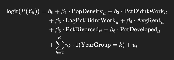{fig-alt="Distress presence predictive logit mixed-effects model."}Where:* β~0~ -> fixed intercept* β~1~,…,β~6~ -> fixed-effect coefficients* γ~k~γ~k~ -> fixed effects for year group (excluding the reference group)* u~i~ -> random intercept for block group i (GEOID)Before interpretation and result analysis can be conducted, various diagnostic tests must be completed to ensure model stability and fit.### Diagnostic Testing```{r diagnostic_testing, message = FALSE, warning = FALSE}#| cache: false# residual diagnostics by simulating residuals to check for# uniformity, outliers, non-linearity, and heterscedasticity# simulate residualssim_res <- simulateResiduals(model_glmm)# plot simulated residualsplot(sim_res)# check for zero inflationtestZeroInflation(sim_res)# check for normality of random effects,# then plot a histogram of themranef_vals <- ranef(model_glmm)$cond$GEOIDggplot(data.frame(ranef = ranef_vals[,1]), aes(x = ranef)) + geom_histogram(bins = 30) + labs(title = 'Distribution of Random Intercepts (GEOID)', x = 'Random Effects', y = 'Count')# approximate multicollinearityvif_check <- lm( is_distressed ~ tot_pop_density + pct_didnt_work_past_yr + lag_pct_didnt_work_past_yr + avg_rent + pct_divorced + pct_developed + factor(year_group), data = train_data)vif(vif_check)#### Moran's I (spatial autocorrelation)#### train_bgs <- train_data %>% distinct(GEOID, .keep_all = TRUE)unique_train_geoids <- unique(train_bgs$GEOID)# extract residuals and attach GEOID, calculate avg residuals per block group,# then ensure order matches spatial weights matrixavg_res <- data.frame( GEOID = train_data$GEOID, residuals = residuals(model_glmm)) %>% group_by(GEOID) %>% summarize(mean_residual = mean(residuals, na.rm = TRUE)) %>% arrange(match(GEOID, unique_train_geoids))# get centroids of unique block groupscentroids_train <- st_centroid(train_bgs)coords_train <- st_coordinates(centroids_train)[, 1:2]# define k-nearest neighborsknn_neighbors_train <- knearneigh(coords_train, k = k)nb_train <- knn2nb(knn_neighbors_train)# create spatial weights matrixlw_train <- nb2listw(nb_train, style = 'W')# Moran's I testmoran_test <- moran.test(avg_res$mean_residual, lw_train)moran <- data.frame( Moran_I = moran_test$estimate[[1]], Moran_I_Std_Dev = moran_test$statistic, p_value = moran_test$p.value)moran %>% gt() %>% tab_header( title = 'Moran\'s I Test Results' ) %>% #fmt_markdown(columns = c(CI)) %>% cols_label( Moran_I = 'Moran\'s I', Moran_I_Std_Dev = 'Std. Dev.', p_value = 'p-value' ) %>% tab_options( table.font.size = 'large' )```The KS test result for uniformity showed no significant deviation from uniformity (p = 0.547), which suggests expected well-behaved residuals. The dispersion test showed no significant over- or under-dispersion (p = 0.08), signalling appropriate levels of variance. The outlier test showed no significant outliers (p = 0.645). The zero inflation test showed no evidence of zero inflation (p = 0.512). The QQ plot indicates appropriate residual distribution, and the Residuals vs. Predicted plot shows a slight curve at higher predictions, but is generally fairly flat otherwise. All VIF values used to measure multicollinearity are less than 5, meaning there is no concerning multicollinearity between the predictors.While significant spatial autocorrelation is present in the residuals (Moran's I = 0.088, p < 0.001), its magnitude is modest and expected given the spatial clustering of socioeconomic distress. In precursor models, Moran's I reached upwards of 0.15. The inclusion of a lagged variable and block group-level random effects substantially reduced spatial dependence compared to these initial models.Overall, the model fits well, the random effects have a reasonable distribution, and multicollinearity is not a concern. While spatial autocorrelation is present, it is moderate and characteristic of socioeconomic spatial data. There were also attempts at limiting spatial autocorrelation in the form of introducing a spatially lagged covariate, which alleviated some of the autocorrelation. Remaining autocorrelation likely reflects unmeasured spatial processes beyond the scope of this analysis.### Fixed Effects```{r fixed_effects, message=F, warning=F}#| cache: false# extract fixed effectsfixef_vals <- fixef(model_glmm)$condodds_ratios <- exp(fixef_vals)# get standard errorsse_vals <- summary(model_glmm)$coefficients$cond[, 'Std. Error']# compute 95% confidence intervallower_ci <- exp(fixef_vals - 1.96 * se_vals)upper_ci <- exp(fixef_vals + 1.96 * se_vals)# get fixed effects datafixed_effects <- data.frame( Estimate = fixef_vals, Odds_Ratio = odds_ratios, CI_Lower = lower_ci, CI_Upper = upper_ci, p_value = summary(model_glmm)$coefficients$cond[, 'Pr(>|z|)'] )# odds ratio tableodds_table <- fixed_effects %>% mutate( Predictor = rownames(.), Estimate = round(Estimate, 3), Odds_Ratio = round(Odds_Ratio, 2), CI = paste0('[', round(CI_Lower, 2), ', ', round(CI_Upper, 2), ']'), p_value = formatC(p_value, format = 'e', digits = 2) ) %>% select(Predictor, Estimate, Odds_Ratio, CI, p_value) %>% gt() %>% tab_header( title = 'Odds Ratios from Logit Mixed-Effects Model', subtitle = '95% Confidence Intervals and p-values' ) %>% fmt_markdown(columns = c(CI)) %>% cols_label( Predictor = 'Predictor', Odds_Ratio = 'Odds Ratio', CI = '95% CI', p_value = 'p_value' ) %>% tab_options( table.font.size = 'small', heading.align = 'left' )odds_table# add significance to highlight predictors that are significantfixed_effects.plt_df <- fixed_effects %>% mutate( Predictor = rownames(.), Significance = ifelse(p_value < 0.05, 'Significant', 'Non Significant') )# plot fixed effects with confidence intervals and significancefixed_effects_plt <- ggplot(fixed_effects.plt_df, aes(x = reorder(Predictor, Odds_Ratio), y = Odds_Ratio)) + geom_point(aes(color = Significance), size = 3) + geom_errorbar(aes(ymin = CI_Lower, ymax = CI_Upper, color = Significance), width = 0.2) + geom_hline(yintercept = 1, linetype = 'dashed', color = 'red') + scale_y_log10() + # log scale for more condense plot coord_flip() + labs( title = 'Odds Ratios with 95% Confidence Intervals', subtitle = 'Logit Mixed-Effects Model (glmmTMB) with Spatial Lag', x = 'Predictor', y = 'Odds Ratio (log scale)', color = 'Significance' )fixed_effects_plt```The fit statistics (AIC = 3595.7, BIC = 3669.7, Log-Likelihood = -1787.8) suggests that the model is well-fitting given the number of predictors and amount of data. Since all predictors were scaled (i.e., standardized), interpretations are based on 1 standard deviation changes. Population density, unemployment rate, divorced rate, and percentage developed land cover are all strong, statistically significant predictors of distress and are all associated with a large increased odds that a block group is distressed. The highly increased odds of distress associated with higher population density and percentage developed land cover suggests that denser development and urbanization play a significant role in distress. At the same time, average rent plays the role of a minor yet statistically significant protective factor and would suggest that a block group with higher rent may be more stable. The 2019-2023 year group is statistically significant, which shows that a trend of higher distressed odds started especially after 2018. This would suggest that various socioeconomic factors have gotten worse in the Southern Tier at least since 2018, leading to increased distress across the region over time and may have been exacerbated (or even caused) by the COVID pandemic.Distress risk is not just temporal. The spatially lagged covariate of unemployment rate is also a strong, significant predictor of distress. It suggests that higher rates of unemployment in neighboring block groups are strongly associated with increased odds of distress in a given block group. More specifically, a 1 standard deviation increase in the spatially lagged unemployment rate is associated with a threefold increase in the odds that a block group is classified as distressed, independent of its own unemployment rate. Even if a block group's own unemployment is more moderate, being surrounded by high-unemployment areas still substantially increases distress risk.### Model Prediction AccuracyA confusion matrix is created from predicted probabilities that are converted to binary predictions, and then the model's overall accuracy, sensitivity, and specificity are calculated by using the remaining 20% of unique block group GEOIDs as test data.```{r model_accuracy, message=F, warning=F}#| cache: false# get predicted probabilitiespred_probs <- predict(model_glmm, newdata = test_data, type = 'response', allow.new.levels = TRUE)# convert probabilities to binary predictionspred_class <- ifelse(pred_probs > 0.5, 1, 0)# create confusion matrix, then extract valuesconf_matrix <- table(Predicted = pred_class, Actual = test_data$is_distressed)TN <- conf_matrix[1,1]FP <- conf_matrix[2,1]FN <- conf_matrix[1,2]TP <- conf_matrix[2,2]# create confusion matrix dataframeconfusion_df <- tibble( Outcome = c('True Negatives', 'False Positives', 'False Negatives', 'True Positives'), Count = c(TN, FP, FN, TP))# create gt table for confusion matrixconfusion_gt <- confusion_df %>% gt() %>% tab_header(title = 'Confusion Matrix: Distressed Status Prediction Model') %>% fmt_number(columns = Count, decimals = 0)# calculate metricsaccuracy <- (TP + TN) / sum(conf_matrix)sensitivity <- TP / (TP + FN)specificity <- TN / (TN + FP)# create metrix dataframemetrics_df <- tibble( Metric = c('Accuracy', 'Sensitivity (Recall)', 'Specificity'), Value = c(accuracy, sensitivity, specificity))# create gt table for metricsmetrics_gt <- metrics_df %>% mutate(Value = round(Value, 4)) %>% gt() %>% tab_header(title = 'Distressed Status Prediction Model Performance Metrics') %>% fmt_percent(columns = Value, decimals = 2)# show gt tables of confusion matrix and metricsconfusion_gtmetrics_gt```Overall, the model has a prediction accuracy rate of about 92%. However, this is mostly due to the model's high level of ability at ruling out distress evidenced by its 99% specificity. Accuracy suffers substantially at predicting block groups that are in distress, where it is only ~28% accurate. This suggests that the model is conservative and is extremely cautious about labeling a block group as distressed unless strong evidence is present. The pattern of false negatives is in line with the fact that distressed areas are a bit rare in the data and the model prioritizes minimizing false positives over catching all distress cases.### Random Effects (Evaluate Areas with Unexpectedly High Risk of Distress)```{r random_effects, message=T, warning=T}#| cache: false# get ordered unique GEOIDsgeoid_levels <- unique(model_glmm$frame$GEOID)# extract random effects (each unique GEOID and its random intercept)ranef_data <- ranef(model_glmm)$cond$GEOID %>% as_tibble() %>% mutate(GEOID = geoid_levels) %>% rename(random_intercept = `(Intercept)`) %>% relocate(GEOID, .before = random_intercept)# join random effects to block groupsst_bgs.ranef <- st_bgs_all %>% distinct(GEOID, .keep_all = TRUE) %>% left_join(ranef_data, by = 'GEOID') #mutate(region = sapply(county, get_region)) %>% #relocate(region, .after = county)# make map of random effects to see which aras have a higher unexplained risk of# being distressed due to reasons not measured in the modelranef_map <- ggplot() + geom_sf(data = st_bgs.ranef, aes(fill = random_intercept), color = NA) + geom_sf(data = st_full_study_area, color= 'grey80', fill = NA, linewidth = 0.1) + geom_sf_text(data = cities, aes(label = NAME), angle = 22.5, size = 3.75) + geom_sf_text(data = civil, aes(label = NAME), angle = -22.5, size = 3) + scale_fill_gradientn( colors = c('darkblue', 'white', 'red'), values = rescale(c(min(st_bgs.ranef$random_intercept, na.rm = T), -3, 3, max(st_bgs.ranef$random_intercept, na.rm = T))), limits = c(min(st_bgs.ranef$random_intercept), max(st_bgs.ranef$random_intercept)), oob = squish, name = 'Random Intercept\n(Log-Odds)', na.value = 'white' ) + labs( title = 'Unexplained Distress Risk by Block Group', subtitle = 'Baseline Distress Risk After Controlling for Predictors' ) + theme_map() + theme( plot.margin = margin(10, 10, 10, 10), legend.position = 'bottom' ) + guides(fill = guide_legend(nrow = 1)) + coord_sf(expand = FALSE)ranef_map```A variance of 8.415 and standard deviation of 2.901 in the random effects show a high level of between-group variability, which suggests that unobserved block group-level factors play a large role in predicting distress in this model. It was thus justified to include the random intercepts to account for this heterogeneity.The map highlights spatial variation in unexplained distress risk across block groups. Several areas of the Southern Tier exhibit significantly higher baseline distress risk (in red) even after controlling for socioeconomic, demographic, and built environment predictors. This suggests the presence of unmeasured local factors contributing to persistent distress. Conversely, pockets of lower-than-expected risk (in blue) indicate potential resilience factors that buffer against socioeconomic vulnerabilities. These spatial patterns warrant further investigation to identify contextual drivers of distress beyond those captured in the current model, as well as methods and policy implementations that could potentially offset the effects of poverty, unemployment rate, and other socioeconomic conditions.Most of the larger cities in the Southern Tier (Binghamton, Jamestown, Ithaca, and Elmira) and other urban centers (such as Oneonta and Olean) express a particular "urban divide" among its census tracts, where pockets of neighborhoods have lower-than-expected distress risk and others have higher-than-expected distress risk. There is also an urban/suburban divide between more stable suburban block groups and socioeconomically vulnerable urban block groups. A vast majority of the higher-risk block groups were urban in nature. A handfull of rural areas in each county exhibited higher-than-expected distress risk, including the entirety of the Allegany Indian Reservation centered around the small but vulnerable urban core of Salamanca. Still, urban cores were significantly more likely to be distressed than rural areas.# Discussion and ConclusionsThe model revealed several statistically significant predictors of distress that align with and extend existing literature on rural vulnerability. Notably, the percentage of individuals not working in the past year emerged as a robust predictor, with both a block group’s own unemployment rate and the spatially lagged rate in neighboring areas being associated with significantly increased odds of having distressed status. This finding underscores the importance of accounting for spatial spillover effects; communities do not exist in isolation, and economic hardship in one area often correlates with, and potentially contributes to, hardship in adjacent areas. The spatial lag term specifically highlights the diffusive nature of socioeconomic stress, validating recent methodological recommendations to include spatial structure in GLMMs (Dormann et al., 2007; Zuur et al., 2009).In addition, the model identified population density, divorce rate, and urban development intensity as significant positive predictors of distress. These findings complicate conventional narratives that associate urbanization and density with economic opportunity. In the context of the Southern Tier, where many small cities and formerly industrial urban areas have suffered from long-term economic decline, these variables may reflect concentrated disadvantage, aging population and/or infrastructure, and systemic disinvestment. Conversely, higher average rent was associated with slightly lower odds of distress, potentially serving as a proxy for neighborhood stability or housing demand, although the effect was relatively modest.The inclusion of year-group fixed effects also confirmed a significant temporal shift: block groups in the 2019–2023 period were far more likely to be classified as distressed, even after accounting for structural and spatial factors. This supports evidence that distress risk has especially been increasing in recent years, likely due to COVID-19 disruptions, continued population decline, and limited regional economic diversification.Despite the strong predictive performance of the model, which achieved an accuracy rate of 92% and a specificity above 99%, some limitations remain. Sensitivity was lower at ~28%, suggesting that an overwhelming majority of distressed block groups may remain undetected by the model. These false negatives could reflect areas where unmeasured protective factors or data limitations obscure underlying distress. Additionally, spatial autocorrelation remains present in the residuals, indicating that the model may not fully capture all spatial dependencies. Incorporating spatially structured random effects or moving toward spatial error models may be necessary to account for latent clustering in future research.Moreover, the method of interpolating variables across changing block group boundaries introduces further limitations. This study used population-weighted areal interpolation through centroid assignment which may produce bias in high-variance areas. As Hallisey et al. (2017) note, centroid-based interpolation can contribute to large absolute errors in count data. Future work could explore hybrid approaches, including combined population and areal weighting or dasymetric interpolation using ancillary data like land cover, to enhance spatial accuracy.By applying the ARC’s Distressed Areas Classification System at the census block group level, this study tested its efficacy in identifying localized socioeconomic vulnerability. While the ARC’s original formulation is effective for broader regional comparisons, it may miss important within-county variation in distress patterns, particularly in geographically and demographically heterogeneous areas like the Southern Tier. The results suggest that the ARC's thresholds alone (67% of national median family income and 150% of the national poverty rate) do not identify many of the most vulnerable communities. The random intercepts in the GLMM, which are interpreted as "unexplained" risk after accounting for observed predictors, revealed significant residual variation across block groups. In other words, certain block groups experienced higher or lower distress risk than would be predicted solely from ARC-defined economic indicators and the model’s covariates.Mapping these random intercepts revealed both inter-county variation and stark intra-urban disparities. While rural pockets in counties like Allegany, Delaware, and Schuyler exhibited elevated unexplained distress, several cities (including Binghamton, Ithaca, Jamestown, Elmira, and Oneonta) showed a pronounced internal divide. In these cities, some block groups had much higher-than-expected baseline distress risk, while adjacent ones had negative random effects, indicating lower-than-expected risk. This “urban divide” suggests that distress may concentrate in historically segregated or economically isolated neighborhoods within cities, reinforcing the idea that urban centers in rural regions are not uniformly distressed but fractured by block-level variation in resilience, opportunity, and historical disinvestment. These observations raise important questions about the adequacy of county-averaged or citywide metrics for targeting interventions. While the ARC’s framework provides a valuable starting point, the findings here emphasize the value of block group-level analysis to surface hidden pockets of vulnerability or resilience that are invisible at coarser scales.To build on these insights, future analyses should explore additional explanatory variables. Potential protective factors may include social capital (e.g., volunteerism, civic engagement), access to green space, proximity to community services, or the presence of mutual aid networks. Structural variables such as redlining history, credit access, school quality, or broadband availability may also help explain residual variation. For instance, changes in volunteerism over time, particularly during crises, offer natural experiments that could be exploited to assess causal effects on community vulnerability. Studies like Makridis and Wu (2021) have demonstrated that counties with greater civic engagement and volunteerism had stronger economic resilience during the COVID-19 pandemic, suggesting shifts in social capital could be causally linked to socioeconomic outcomes. Additionally, the sudden expansion of mutual aid networks during the pandemic provides a quasi-experimental setting to evaluate whether localized increases in social support structures reduced vulnerability. One such study by Xu and Zhang (2025) utilized structural equation modeling to analyze data from participants in mutual aid groups in China during the pandemic. The research found that participation in mutual aid significantly enhanced individuals' subjective well-being. This effect was mediated through increased access to material resources and the expansion of social networks, which in turn boosted self-esteem and self-efficacy. The study highlights the mechanisms by which mutual aid can reduce vulnerability and promote resilience in times of crisis.Integrating dynamic measures—such as industry closures, pandemic impacts, or population churn—could further improve temporal responsiveness and causal interpretation. For example, differences-in-differences designs exploiting the staggered rollout of broadband access across rural areas (Bertschek et al., 2016) could be adapted to assess how changes in structural resources affect economic distress trajectories. Methodologically, sensitivity could be improved through more flexible classification thresholds, bootstrapped uncertainty intervals, or temporal interaction terms. Moving beyond cross-sectional associations to leverage these natural variations would offer stronger evidence on causal pathways and actionable intervention points.This study contributes to a growing body of research calling for more spatially nuanced approaches to understanding and addressing rural economic distress. By integrating predictive modeling with the ARC classification framework, it underscores both the value and the limitations of existing policy tools and demonstrates the power of glmmTMB-based modeling for applied regional analysis. The inclusion of spatial random effects and the visual analysis of residuals provide a roadmap for targeting interventions more precisely, improving both the scientific understanding and the policy relevance of distress classification systems.```{=latex}\newpage```# References## Works Cited1. Appalachian Regional Commission. (2023). County Economic Status and Distressed Areas by State, FY 2024. <https://www.arc.gov/about-the-appalachian-region/county-economic-status-and-distressed-areas-by-state-fy-2024>2. Appalachian Regional Commission. (2024). Distressed Areas Classification System. <https://www.arc.gov/distressed-areas-classification-system/>3. Barrett, M., Aslebagh, S., Vuong, V., et al. (2023). Spatially resolved air pollution models identify disparities in exposure by socioeconomic status. *European Respiratory Journal*, *62*(67). <https://doi.org/10.1183/13993003.congress-2023.PA1608>4. Bertschek, I., Briglauer, W., Hüschelrath, K., Kauf, B., & Niebel, T. (2016). The Economic Impacts of Broadband Internet: A Survey. *Review of Network Economics*, *14*(4), 201–227. <https://doi.org/10.1515/rne-2016-0032>5. Bivand, R. S., & Piras, G. (2015). Comparing implementations of estimation methods for spatial econometrics. Journal of Statistical Software, *63*(18), 1–36. <https://doi.org/10.18637/jss.v063.i18>6. Brooks M.E., Kristensen K., van Benthem K.J., et al. (2017). glmmTMB Balances Speed and Flexibility Among Packages for Zero-inflated Generalized Linear Mixed Modeling. *The R Journal*, *9*(2), 378–400. <https://doi.org/doi:10.32614/RJ-2017-066>.7. Dormann, C. F., McPherson, J. M., Araújo, M. B., et al. (2007). Methods to account for spatial autocorrelation in the analysis of species distributional data: A review. *Ecography*, *30*(5), 609–628. <https://doi.org/10.1111/j.2007.0906-7590.05171.x>8. Ellis, G.F., Burk, D., Roberts, F. (2025). ipumsr: An R Interface for Downloading, Reading, and Handling IPUMS Data. R package version 0.8.2, <https://github.com/ipums/ipumsr>, <https://www.ipums.org>, <https://tech.popdata.org/ipumsr/>. 9. Flowerdew, R., & Green, M. (1992). Developments in areal interpolation methods and GIS. The Annals of Regional Science, 26(1), 67–78. <https://doi.org/10.1007/BF01581870>10. Galili, T., O'Callaghan, A., Sidi, J., & Sievert, C. (2017). heatmaply: an R package for creating interactive cluster heatmaps for online publishing. *Bioinformatics*, *34*(9), 1600-1602. <https://doi.org/10.1093/bioinformatics/btx657>11. Gelman, A. & Hill, J. (2007). Data Analysis Using Regression and Multilevel/Hierarchical Models. Cambridge University Press. <https://doi.org/10.1017/CBO9780511790942>12. Goodchild, M. F., & Lam, N. S. (1980). Areal interpolation: A variant of the traditional spatial problem. *Geo-Processing*, *1*(3), 297-312. <https://www.researchgate.net/publication/239654534_Areal_Interpolation_A_Variant_of_the_Traditional_Spatial_Problem>13. Gregory, I. N. (2002). The accuracy of areal interpolation techniques: standardising the crosswalk. *Computers, Environment and Urban Systems*, *26*(3), 293-314. <https://www.researchgate.net/publication/223083878_The_accuracy_of_areal_interpolation_techniques_Standardising_19th_and_20th_century_census_data_to_allow_long-term_comparisons>14. Hallisey, E., Tai, E., Berens, A., et al. (2017). Transforming geographic scale: a comparison of combined population and areal weighting to other interpoaltion methods. *International Journal of Health Geographics*, *16*(29). <https://doi.org/10.1186/s12942-017-0102-z>15. Hartig, F. (2024). DHARMa: Residual Diagnostics for Hierarchical (Multi-Level / Mixed) Regression Models. R package version 0.4.7, <https://github.com/florianhartig/dharma>.16. Hijmans, R. (2025). terra: Spatial Data Analysis. R package version 1.8-6. <https://github.com/rspatial/terra>17. Johnson, K. M., & Lichter, D. T. (2019). Rural depopulation: Growth and decline processes over the past century. Rural Sociology, 84(1), 3–27. <https://doi.org/10.1111/ruso.12266>18. Jokela, M., Batty, G. D., Vahtera, J., Elovainio, M., & Kivimäki, M. (2013).Socioeconomic inequalities in common mental disorders and psychotherapy treatment in the UK between 1991 and 2009. The British Journal of Psychiatry, 202(2), 115–120. <https://doi.org/10.1192/bjp.bp.111.098863>19. K C, S., Gyawali, B. R., Lucas, S., Antonious, G. F., Chiluwal, A., & Zourarakis, D. (2024). Assessing Land-Cover Change Trends, Patterns, and Transitions in Coalfield Counties of Eastern Kentucky, USA. *Land*, *13*(9), 1541. <https://doi.org/10.3390/land13091541>20. Ludke, R. L., Obermiller, P. J., & Rademacher, E. W. (2012). Demographic Change in Appalachia: A Tentative Analysis. *Journal of Appalachian Studies*, *18*(1/2), 48–92. <http://www.jstor.org/stable/23337708>21. Makridis, C. A. & Wu, C. (2021). How social capital helps communities weather the COVID-19 pandemic. *PLOS ONE*, *16*(1). <https://doi.org/10.1371/journal.pone.0245135>22. Manson, S., Schroeder, J., Van Riper, D., et al. (2024). IPUMS National Historical Geographic Information System: Version 19.0 [dataset]. Minneapolis, MN: IPUMS. <http://doi.org/10.18128/D050.V19.0>.23. McMahon, E.J. (2024). Eight in 10 New York towns and cities have lost population since 2020. *Empire Center*. <https://www.empirecenter.org/publications/eight-in-10-new-york-towns-and-cities-have-lost-population-since-2020>24. Partridge, M. D., Rickman, D. S., Ali, K., & Olfert, M. R. (2008).Lost in space: Population growth in the American hinterlands and small cities.Journal of Economic Geography, 8(6), 727–757.<https://doi.org/10.1093/jeg/lbn038>25. Thiede, B. C., Lichter, D. T., & Slack, T. (2018). Working, but poor: The good life in rural America? Journal of Rural Studies, 59, 183–193. <https://doi.org/10.1016/j.jrurstud.2016.02.007>26. U.S. Geological Survey. (2024). Annual National Land Cover Database (NLCD) Collection 1 Science Products (2008–2023) [Data set]. Multi-Resolution Land Characteristics Consortium ([MRLC](https://www.mrlc.gov/sites/default/files/docs/LSDS-2103%20Annual%20National%20Land%20Cover%20Database%20%28NLCD%29%20Collection%201%20Science%20Product%20User%20Guide%20-v1.0%202024_10_15.pdf)).27. Walker, K. (2023). "7.3 Small area time-series analysis," in *Analyzing US Census Data: Methods, Maps, and Models in R*. CRC Press: Boca Raton, Florida, <https://walker-data.com/census-r/spatial-analysis-with-us-census-data.html#small-area-time-series-analysis>28. Walker, K. & Herman, M. (2024). tidycensus: Load US Census Boundary and Attribute Data as 'tidyverse' and 'sf'-Ready Data Frames. R package version 1.6.6. <https://walker-data.com/tidycensus>29. Xu, A., & Zhang, Y. (2025). The effect and mechanism of mutual aid on the subjective well-being of participants under the COVID-19 pandemic. BMC Psychology, 13, Article 48. https://doi.org/10.1186/s40359-025-02360-530. Zuur, A. F., Ieno, E. N., Walker, N. J., Saveliev, A. A., & Smith, G. M. (2009). Mixed Effects Models and Extensions in Ecology with R. Springer Science & Business Media. <https://doi.org/10.1007/978-0-387-87458-6>```{=latex}\newpage```## Data Sources and Methodology[2009 U.S. Data]{.underline}* Total Population: <https://api.census.gov/data/2009/acs/acs5?get=B02001_001E,NAME&for=us>* Median Family Income: U.S. Department of Housing and Urban Development. (19 March 2009). "Estimated Median Family Incomes for Fiscal Year 2009," PDR-2009-01. <https://www.huduser.gov/portal/datasets/il/il09/Medians2009.pdf>* Poverty Rate: Bishaw, A. & Macartney, S. (September 2010). "Poverty: 2008 and 2009," American Community Survey Briefs, ACSBR/09-1. U.S. Census Bureau, Washington, D.C. <https://www2.census.gov/library/publications/2010/acs/acsbr09-01.pdf>[2010 U.S. Data]{.underline}* Total Population: U.S. Census Bureau. (2010). 2010 Summary File 1 Tables [All 50 States & DC]. <https://api.census.gov/data/2010/dec/sf1?>* Median Family Income: U.S. Department of Housing and Urban Development. (14 May 2010). "Estimated Median Family Incomes for Fiscal Year 2010," PDR-2010-01. <https://www.huduser.gov/portal/datasets/il/il10/Medians2010.pdf>* Poverty Rate: Bishaw, A. (September 2012). "Poverty: 2010 and 2011," American Community Survey Briefs, ACSBR/11-01. U.S. Census Bureau, Washington, D.C. <https://www2.census.gov/library/publications/2012/acs/acsbr11-01.pdf>, pg. 3.* 2009 & 2010 Per Capita Income and Haven't Worked Population: [U.S. Bureau of Economic Analysis](https://apps.bea.gov/iTable/?reqid=70&step=30&isuri=1&major_area=0&area=xx&year=2018,2017,2016,2015,2014,2013,2012,2011,2010,2009,2008,2007,2006,2005,2004,2003,2002,2001,2000,1999,1998,1997,1996&tableid=21&category=421&area_type=0&year_end=-1&classification=non-industry&state=0&statistic=3&yearbegin=-1&unit_of_measure=levels).[American Community Survey (ACS) Data]{.underline}* U.S. Census Bureau. (2009-2023). American Community Survey 5-Year Estimates: Comparison Profiles 5-Year. <http://api.census.gov/data/2010/acs/acs5>* U.S. Census Bureau. (2010). "Selected Economic Characteristics." American Community Survey 5-Year Estimates Subject Tables, Table DP03. <https://data.census.gov/table/ACSDP5YSPT2010.DP03>* U.S. Census Bureau. (2019). "Selected Economic Characteristics." American Community Survey 5-Year Estimates Subject Tables, Table DP03. <https://data.census.gov/table/ACSDP5Y2019.DP03>[Land Cover Data]{.underline}* U.S. Geological Survey (USGS). (2008-2023). Annual National Land Cover Data Collection 1 Science Products: U.S. Geological Survey data releases. Data downloaded from: <https://www.mrlc.gov/data?f[0]=category%3ALand%20Cover>* Land Cover Classifications from the [Multi-Resolution Land Characteristics Consortium](https://www.mrlc.gov/data/type/land-cover)


